6 Statistical analysis

Learning Objectives

Know how to filter proteins for statistical testing based on quantification across replicates
Using the limma package (Smyth (2004)), design a statistical model with contrasts to test for differentially abundant proteins across multiple conditions
Understand the F-test for overall significance across groups
Interpret the results of individual pairwise contrasts and apply global multiple testing correction
Produce volcano plots to visualise the results of differential abundance analysis

6.1 Differential abundance analysis

Having cleaned our data, aggregated from precursor to protein level, log2 transformed and normalised, we are now ready to carry out statistical analysis.

The aim of this section is to answer the question: “Which proteins show a significant change in abundance between MPXV-infected patients, COVID-19 patients, and healthy controls?”.

Our null hypothesis is: (H0) The mean protein abundance is the same across all three groups.

Our alternative hypothesis is: (H1) The mean protein abundance differs between at least one pair of groups.

6.2 Selecting a statistical test

There are a few aspects of our data that we need to consider prior to deciding which statistical test to apply.

The protein abundances in this data are not normally distributed (i.e., they do not follow a Gaussian distribution). However, they are approximately normal following a log-transformation.
We assume that the variance is approximately equal across the three groups.
The samples are independent and not paired — each patient contributes a single sample to one group only.

The first point relates to a key assumption of Gaussian linear modelling, which assumes that the residuals (difference between the observed values and the values predicted by the model) are Gaussian distributed. If this assumption is not met, it is not appropriate to use a Gaussian linear model. For quantitative proteomics data, it is reasonable to assume the residuals will be approximately Gaussian distributed if we first log-transform the abundances.

Many different R packages can be used to carry out differential abundance analysis on proteomics data. Here we will use limma, a package that is widely used for omics analysis and can be used in single comparisons or multifactorial experiments using an empirical Bayes-moderated linear model. A simple example of the empirical Bayes-moderated linear model is provided in Hutchings et al. (2024).

6.2.1 What does the empirical Bayes part mean?

When carrying out high throughput omics experiments we not only have a population of samples but also a population of features - here we have several thousand proteins. Proteomics experiments are typically lowly replicated (e.g n < 10), therefore, the per-protein variance estimates are relatively inaccurate. The empirical Bayes method borrows information across features (proteins) and shifts the per-protein variance estimates towards an expected value based on the variance estimates of other proteins with a similar abundance. This improves the accuracy of the variance estimates, thus reducing false negatives for proteins with over-estimated variance and reducing false positives from proteins with under-estimated variance. For more detail about the empirical Bayes methods, see here.

6.3 Handling missing values prior to testing

DIA data contains a higher proportion of missing values than TMT data. Before statistical testing, we need to decide how to handle proteins that are not quantified in enough samples within each group to support a reliable estimate of group-level abundance.

We only want to test proteins which are quantified in at least 3 replicates of each condition. We first split the data by group, then count the number of finite (non-missing) values per protein within each group.

We begin by extracting the normalised protein level data "norm_protiens" in the QF object.

se <- getWithColData(dia_qf, "norm_proteins")
print(se)

class: SummarizedExperiment 
dim: 368 31 
metadata(0):
assays(2): assay aggcounts
rownames(368): A0A075B6H7;A0A0C4DH90;A0A0C4DH55;P01624 A0A075B6H9 ...
  Q9Y5J9 Q9Y6R7
rowData names(22): Channel Decoy ... Lib.PG.Q.Value .n
colnames(31): COVID_E1 COVID_E10 ... MPX_D5 MPX_D6
colData names(5): sample_id runCol group sex age.group

Now let’s subset the dataset by condition,

control <- se[, se$group == "control"]
mpxv    <- se[, se$group == "MPXV"]
cov     <- se[, se$group == "Covid19"]

Finally, we keep only proteins quantified in at least 3 replicates.

control_replicated <- rowSums(!is.na(assay(control))) >= 3
mpxv_replicated    <- rowSums(!is.na(assay(mpxv))) >= 3
cov_replicated     <- rowSums(!is.na(assay(cov))) >= 3 

# Keep proteins common in all conditions
tokeep <- control_replicated & mpxv_replicated & cov_replicated
print(table(tokeep))

tokeep
FALSE  TRUE 
   26   342

We now add a new set containing only the proteins that pass the replication filter, and link it to the parent set.

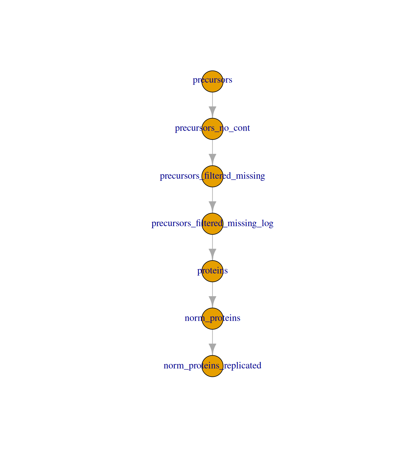
dia_qf <- addAssay(dia_qf, 
                   y = se[tokeep, ],
                   name = "norm_proteins_replicated")

dia_qf <- addAssayLink(dia_qf,
                       from = "norm_proteins",
                       to = "norm_proteins_replicated")

dia_qf

An instance of class QFeatures (type: bulk) with 7 sets:

 [1] precursors: SummarizedExperiment with 4692 rows and 31 columns 
 [2] precursors_no_cont: SummarizedExperiment with 4417 rows and 31 columns 
 [3] precursors_filtered_missing: SummarizedExperiment with 4137 rows and 31 columns 
 [4] precursors_filtered_missing_log: SummarizedExperiment with 4137 rows and 31 columns 
 [5] proteins: SummarizedExperiment with 368 rows and 31 columns 
 [6] norm_proteins: SummarizedExperiment with 368 rows and 31 columns 
 [7] norm_proteins_replicated: SummarizedExperiment with 342 rows and 31 columns

plot(dia_qf)

6.4 Defining the statistical model

We use model.matrix to define the design matrix for our linear model. Since we have three groups and are interested in all pairwise comparisons, we use a model without an intercept (~0 + group). This means the model estimates the mean abundance for each group directly.

group <- factor(dia_qf$group, levels = c("control", "MPXV", "Covid19"))

limma_design <- model.matrix(formula(~0 + group))

# Rename design matrix columns to make them easier to refer to
colnames(limma_design) <- levels(group)

## Verify
limma_design

   control MPXV Covid19
1        0    0       1
2        0    0       1
3        0    0       1
4        0    0       1
5        0    0       1
6        0    0       1
7        0    0       1
8        0    0       1
9        0    0       1
10       0    0       1
11       1    0       0
12       1    0       0
13       1    0       0
14       1    0       0
15       1    0       0
16       1    0       0
17       1    0       0
18       1    0       0
19       1    0       0
20       1    0       0
21       1    0       0
22       1    0       0
23       1    0       0
24       1    0       0
25       1    0       0
26       0    1       0
27       0    1       0
28       0    1       0
29       0    1       0
30       0    1       0
31       0    1       0
attr(,"assign")
[1] 1 1 1
attr(,"contrasts")
attr(,"contrasts")$group
[1] "contr.treatment"

We then define the contrasts — the specific pairwise comparisons we wish to make. The makeContrasts function creates a contrast matrix specifying how differences between group means should be calculated.

## Specify contrasts of interest
contrasts_matrix <- makeContrasts(MPXV_control  = MPXV - control,
                                  Covid19_control = Covid19 - control,
                                  MPXV_Covid19  = MPXV - Covid19,
                                  levels = limma_design)

## Verify
contrasts_matrix

         Contrasts
Levels    MPXV_control Covid19_control MPXV_Covid19
  control           -1              -1            0
  MPXV               1               0            1
  Covid19            0               1           -1

What is an F-value?

An F-value is a parametric statistical value used to compare the mean values of three or more groups. The F-value is the ratio of the between-group variation (explained variance) and the within-group variance (unexplained variance). The higher the F-value, the more significant the difference between the groups is.

What is a t-value?

A t-value is a parametric statistical value used to compare the mean values of two groups. The t-value is the ratio of the difference in means to the standard error of the difference in means. The further away from zero that a t-value lies, the more significant the difference between the groups is.

How is the p-value obtained?

A p-value may be obtained from a t-value/F-value by comparing the value against a t-value/F-distribution with the appropriate degrees of freedom.

degrees of freedom = the number of observations minus the number of independent variables in the model
p-value = the probability of achieving the t-value/F-value under the null hypothesis i.e., by chance

6.5 Running the empirical Bayes-moderated test using `limma`

We fit the linear model to the replicated protein data, apply the contrasts, and then update the model using the eBayes function with trend = TRUE and robust = TRUE to account for the intensity-dependent variance trend typical in quantitative proteomics data.

trend - takes a logical value of TRUE or FALSE to indicate whether an intensity-dependent trend should be allowed for the prior variance (i.e., the population level variance prior to empirical Bayes moderation). This means that when the empirical Bayes moderation is applied the protein variances are not squeezed towards a global mean but rather towards an intensity-dependent trend.
robust - takes a logical value of TRUE or FALSE to indicate whether the parameter estimation of the priors should be robust against outlier sample variances.

See (Phipson et al. (2016) and Smyth (2004)) for further details.

data <- assay(dia_qf[['norm_proteins_replicated']])

limma_fit <- lmFit(data,
                   limma_design)

limma_fit_contrasts <- contrasts.fit(fit = limma_fit, 
                                     contrasts = contrasts_matrix)

limma_fit_contrasts <- eBayes(limma_fit_contrasts, 
                              trend = TRUE, 
                              robust = TRUE)

6.5.1 Diagnostic plots to verify suitability of our statistical model

As with all statistical analysis, it is crucial to do some quality control and to check that the statistical test that has been applied was indeed appropriate for the data. As mentioned above, statistical tests typically come with several assumptions. To check that these assumptions were met and that our model was suitable, we create some diagnostic plots.

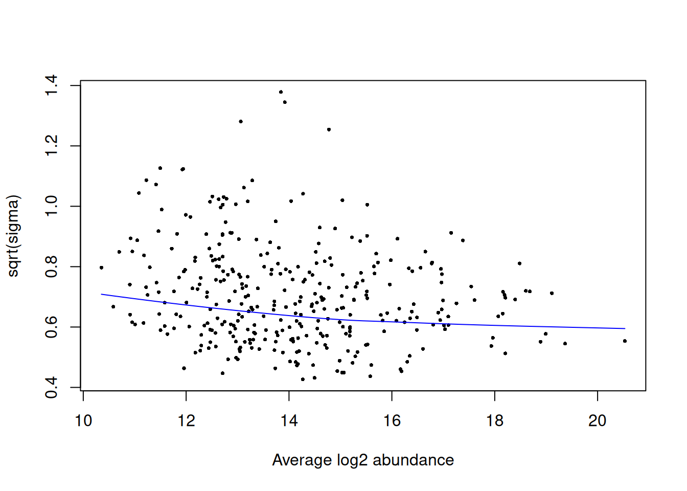
The first plot that we generate is an SA plot to display the residual standard deviation (sigma) versus log abundance for each protein to which our model was fitted. We can use the plotSA function to do this.

plotSA(fit = limma_fit_contrasts,
       cex = 0.5,
       xlab = "Average log2 abundance")

It is recommended that an SA plot be used as a routine diagnostic plot when applying a limma-trend pipeline. From the SA plot we can visualise the intensity-dependent trend that has been incorporated into our linear model. It is important to verify that the trend line fits the data well. If we had not included the trend = TRUE argument in our eBayes function, then we would instead see a straight horizontal line that does not follow the trend of the data. Further, the plot also colours any outliers in red. These are the outliers that are only detected and excluded when using the robust = TRUE argument.

Next, we plot a histogram of the raw p-values (not adjusted p-values). This can be done by passing our results data into standard ggplot2 plotting functions.

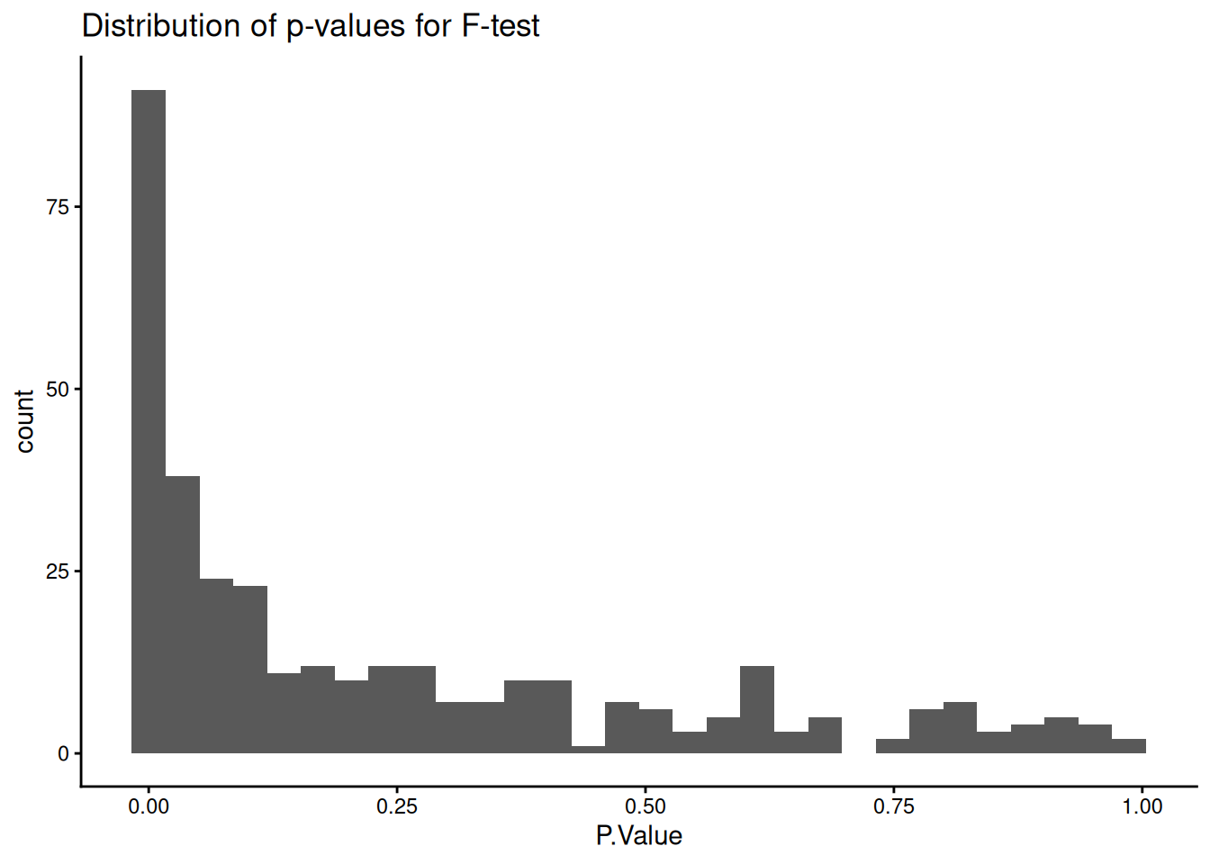
The near-flat distribution across the bottom corresponds to null p-values which are distributed approximately uniformly between 0 and 1. The peak close to 0 contains a combination of our significantly changing proteins (true positives) and proteins with a low p-value by chance (false positives).

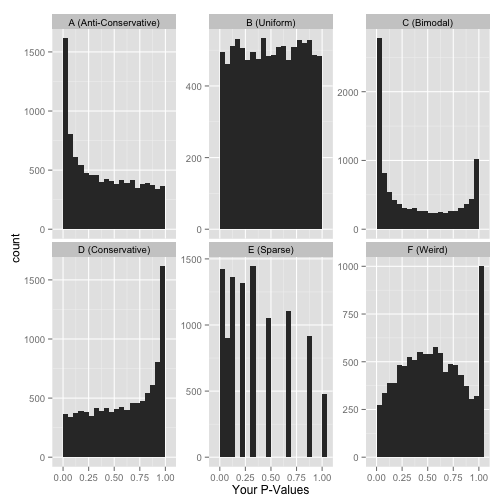
Other examples of how a p-value histogram could look are shown below. Whilst in some experiments a uniform p-value distribution may arise due to an absence of significant alternative hypotheses, other distribution shapes can indicate that something was wrong with the model design or statistical test. For more detail on how to interpret p-value histograms there is a great blog post by David Robinson, from which the examples below are taken.

6.6 F-test for overall significance across groups

Discussion

Before running individual pairwise contrasts, why might it be useful to first test for any significant difference across all groups simultaneously?
What null hypothesis does the F-test test, and how does it differ from a pairwise t-test?
After running the code below, look at the p-value distribution — what shape would you expect if many proteins are truly differentially abundant, and does this plot match your expectation?

We can first test for an overall significant difference across all groups using an F-test. Setting coef = NULL in topTable returns the F-statistic for each protein, which tests the null hypothesis that the mean abundance is equal across all groups.

## Format results
limma_results_F <- topTable(
  fit = limma_fit_contrasts,
  coef = NULL,
  adjust.method = "BH",  # Method for multiple hypothesis testing
  number = Inf) %>%       # Print results for all proteins
  rownames_to_column("UniprotID")

head(limma_results_F)

  UniprotID MPXV_control Covid19_control MPXV_Covid19  AveExpr        F
1    P02766   -1.5515210      -1.6313231   0.07980211 12.95369 75.40937
2    P02652   -1.2644480      -1.4143889   0.14994087 16.42369 35.75869
3    P02654   -3.4780381      -2.5547982  -0.92323989 14.04151 35.43467
4    P05452   -0.7366027      -0.8673067   0.13070396 12.81599 35.38853
5    P02748    1.3808622       1.1927880   0.18807427 14.43917 31.98443
6    P02647   -0.9664780      -1.0782069   0.11172892 18.06976 26.15018
       P.Value    adj.P.Val
1 8.877578e-13 3.036132e-10
2 7.462286e-09 7.151520e-07
3 8.245842e-09 7.151520e-07
4 8.364351e-09 7.151520e-07
5 2.487367e-08 1.701359e-06
6 1.955504e-07 1.114637e-05

# Check distribution of p-values
limma_results_F %>%
  ggplot(aes(x = P.Value)) +
  geom_histogram() +
  theme_classic() +
  ggtitle("Distribution of p-values for F-test")

`stat_bin()` using `bins = 30`. Pick better value `binwidth`.

6.7 Pairwise contrasts

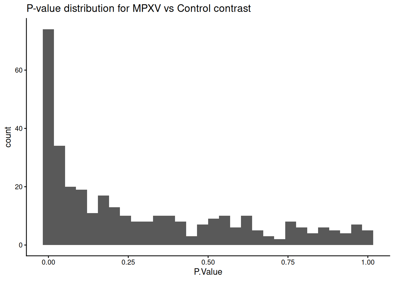
We start by extracting results for a single contrast of particular biological interest: MPXV versus control. We use topTable with coef = "MPXV_control" to get the results for this specific comparison. We also merge in gene name annotations from the rowData.

limma_results_mpxv_control <- topTable(limma_fit_contrasts,
                                       coef = "MPXV_control",
                                       number = Inf,
                                       sort.by = "p") %>%
  data.frame() %>%
  rownames_to_column('UniprotID')

uniprot_annotations <- rowData(dia_qf[['norm_proteins_replicated']]) %>%
  data.frame() %>%
  select(Genes, Protein.Names)

limma_results_mpxv_control <- limma_results_mpxv_control %>%
  merge(uniprot_annotations, by.x = 'UniprotID', by.y = 'row.names') %>%
  arrange(P.Value)

limma_results_mpxv_control %>%
  ggplot(aes(P.Value)) +
  geom_histogram() +
  theme_classic() +
  ggtitle("P-value distribution for MPXV vs Control contrast")

`stat_bin()` using `bins = 30`. Pick better value `binwidth`.

How many significant changes in abundance are there?

table(sig = limma_results_mpxv_control$adj.P.Val < 0.05,
      ifelse(limma_results_mpxv_control$logFC > 0, 'Increased', 'Decreased'))

       
sig     Decreased Increased
  FALSE       136       144
  TRUE         36        26

6.7.1 Multiple hypothesis testing and correction

Using the linear model defined above, we have carried out a statistical test for each protein.

Multiple testing describes the process of separately testing multiple null hypothesis i.e., carrying out many statistical tests at a time, each to test a null hypothesis on different data. Here we have carried out one statistical test per protein. If we were to use the typical p < 0.05 significance threshold for each test, we would expect a 5% chance of incorrectly rejecting the null hypothesis per test. For a typical proteomics dataset with thousands of proteins, we would expect many p-values <= 0.05 by chance.

If we do not account for the fact that we have carried out multiple hypothesis, we risk including false positives in our data. Many methods exist to correct for multiple hypothesis testing and these mainly fall into two categories:

Control of the Family-Wise Error Rate (FWER)
Control of the False Discovery Rate (FDR)

Above we specified the “BH” method for adjusting p-values in our topTable function call. This is shorthand for the Benjamini-Hochberg procedure, to control the FDR.

The False Discovery Rate

The False Discovery Rate (FDR) defines the fraction of false discoveries that we are willing to tolerate in our list of differential proteins. For example, an FDR threshold of 0.05 means that approximately 5% of the proteins deemed differentially abundant will be false positives. It is up to you to decide what this threshold should be, but conventionally a value between 0.01 (1% FPs) and 0.1 (10% FPs) is chosen.

6.8 Visualising results: the volcano plot

The final step in any statistical analysis is to visualise the results. This is important for ourselves as it allows us to check that the data looks as expected.

The most common visualisation used to display the results of expression proteomics experiments is a volcano plot. This is a scatterplot that shows statistical significance (p-values) against the magnitude of fold change. Of note, when we plot the statistical significance we use the raw unadjusted p-value (-log10(P.Value)). This is because it is better to plot the statistical test results in their ‘raw’ form and not values derived from them (the adjusted p-value is derived from each p-value using the BH-method of correction). Furthermore, the process of FDR correction can result in some points that previously had distinct p-values having the same adjusted p-value. Finally, different methods of correction will generate different adjusted p-values, making the comparison and interpretation of values more difficult.

Discussion

What information does a volcano plot convey, and what are its limitations?
Why might some proteins have a large fold change but not be statistically significant?
Look at the proteins near the significance threshold — what does this tell you about treating adj.P.Val < 0.05 as a hard cut-off?

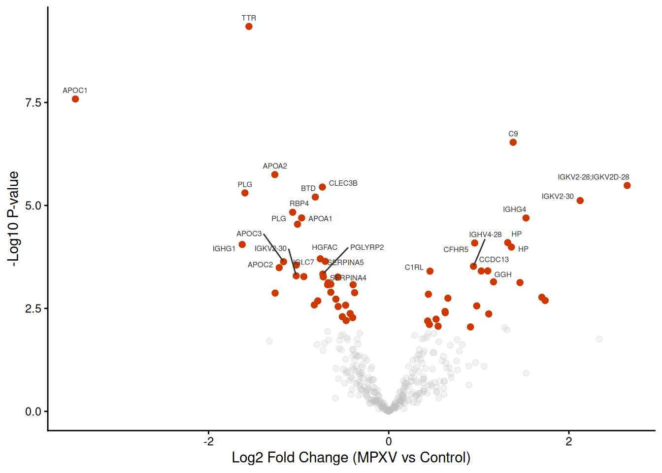
We produce a volcano plot for the MPXV vs Control contrast, labelling the top 30 most significant proteins by gene name.

data_for_highlighting <- limma_results_mpxv_control %>%
  filter(adj.P.Val < 0.05) %>%
  arrange(P.Value) %>%
  head(30)

ggplot(limma_results_mpxv_control,
       aes(logFC, -log10(P.Value),
           colour = adj.P.Val < 0.05,
           alpha = adj.P.Val < 0.05)) +
  geom_point(pch = 20, size = 3) +
  ggrepel::geom_text_repel(
    data = data_for_highlighting,
    aes(label = Genes), vjust = 1.5, size = 2, colour = 'grey20') +
  theme_classic() +
  xlab("Log2 Fold Change (MPXV vs Control)") +
  ylab("-Log10 P-value") +
  scale_colour_manual(values = c('grey', 'orangered3')) +
  scale_alpha_manual(values = c(0.2, 1)) +
  theme(legend.position = "none")

6.9 Extracting results for all contrasts

Rather than extracting results for each contrast separately, we can loop through all contrasts and bind the results into a single long-format data frame. This format is well-suited for downstream visualisation with ggplot2.

contrasts <- colnames(contrasts_matrix)

limma_results_all_contrasts_list <- vector('list', length(contrasts))
names(limma_results_all_contrasts_list) <- contrasts

for(contrast in contrasts){
  limma_results_all_contrasts_list[[contrast]] <- topTable(limma_fit_contrasts,
                                                           coef = contrast,
                                                           number = Inf,
                                                           sort.by = "p") %>%
    data.frame() %>%
    rownames_to_column('UniprotID') %>%
    merge(uniprot_annotations, by.x = 'UniprotID', by.y = 'row.names') %>%
    mutate(contrast = contrast) %>%
    arrange(P.Value)
}

# bind into one data.frame
limma_results_all_contrasts <- bind_rows(limma_results_all_contrasts_list)

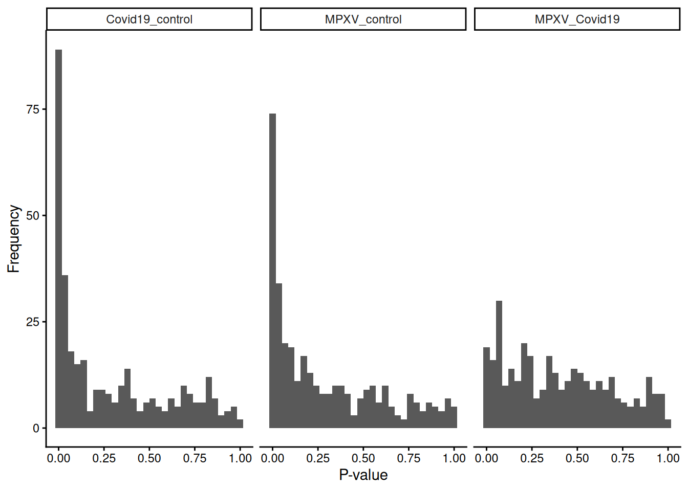
6.9.1 Inspecting p-value distributions across contrasts

Discussion

Before interpreting the results in detail, what can you infer just from the shape of the p-value distributions across the three contrasts?
Which contrast shows the strongest signal, and what does that suggest about the biology?

limma_results_all_contrasts %>%
  ggplot(aes(P.Value)) +
  geom_histogram() +
  theme_classic() +
  labs(x = "P-value", y = "Frequency") +
  facet_wrap(~contrast)

`stat_bin()` using `bins = 30`. Pick better value `binwidth`.

6.9.2 Global multiple testing correction across contrasts

Discussion

Why do we need to adjust p-values when testing thousands of proteins across multiple contrasts?
What is the difference between adjusting each contrast separately versus adjusting globally across all contrasts and proteins?
Which approach is more conservative, and in what circumstances might that matter?

When testing thousands of proteins across multiple contrasts, p-values must be adjusted for multiple testing. The standard Benjamini-Hochberg method was designed for independent tests, but our contrasts share data and are positively correlated. Fortunately, BH remains valid under this kind of positive dependence (formally called Positive Regression Dependency on a Subset, PRDS), so applying BH globally across all contrasts is statistically justified and more rigorous than correcting each contrast separately.

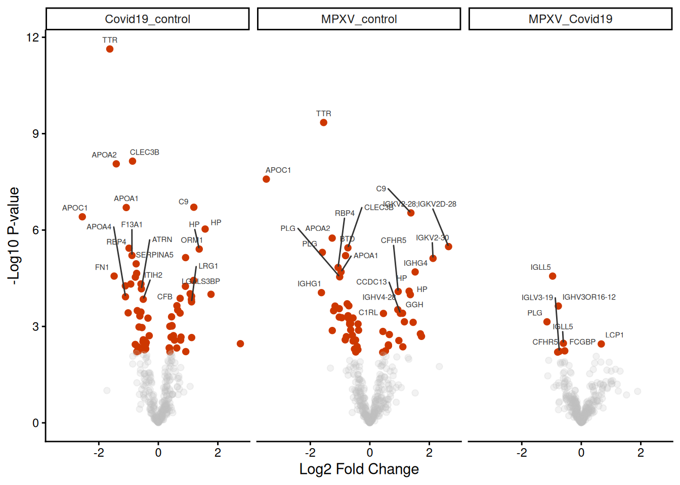
limma_results_all_contrasts <- limma_results_all_contrasts %>%
  mutate(adj.P.Val = p.adjust(P.Value, method = 'BH'))

How many significant changes in abundance are there in each contrast?

Discussion

Looking at the counts of significantly increased and decreased proteins across the three contrasts, what does this tell you about the differences between the conditions?
Are you surprised by any of these numbers? What biological explanations might account for what you see?

table(sig = limma_results_all_contrasts$adj.P.Val < 0.05,
      ifelse(limma_results_all_contrasts$logFC > 0, 'Increased', 'Decreased'),
      limma_results_all_contrasts$contrast)

, ,  = Covid19_control

       
sig     Decreased Increased
  FALSE       111       162
  TRUE         38        31

, ,  = MPXV_control

       
sig     Decreased Increased
  FALSE       136       147
  TRUE         36        23

, ,  = MPXV_Covid19

       
sig     Decreased Increased
  FALSE       178       156
  TRUE          7         1

6.9.3 Volcano plots for all contrasts

data_for_highlighting_all_contrasts <- limma_results_all_contrasts %>%
  filter(adj.P.Val < 0.05) %>%
  arrange(P.Value) %>%
  group_by(contrast) %>% # group by contrast to get top 30 for each contrast
  slice_min(P.Value, n = 30)

ggplot(limma_results_all_contrasts,
       aes(logFC, -log10(P.Value),
           colour = adj.P.Val < 0.05,
           alpha = adj.P.Val < 0.05)) +
  geom_point(pch = 20, size = 3) +
  ggrepel::geom_text_repel(
    data = data_for_highlighting_all_contrasts,
    aes(label = Genes), vjust = 1.5, size = 2, colour = 'grey20') +
  theme_classic() +
  xlab("Log2 Fold Change") +
  ylab("-Log10 P-value") +
  scale_colour_manual(values = c('grey', 'orangered3')) +
  scale_alpha_manual(values = c(0.2, 1)) +
  theme(legend.position = "none") +
  facet_wrap(~contrast) # facet by contrast to get separate volcano plots for each contrast

Exercise 1 - Challenge: Using treat to test against a fold-change threshold

Level:

The eBayes function tests the null hypothesis that a protein’s log fold change is exactly zero. In practice, we are often only interested in changes that exceed a minimum biologically meaningful fold change. The treat function from limma instead tests the null hypothesis that the absolute log fold change is less than a specified threshold fc, providing a statistically rigorous alternative to post-hoc fold-change filtering.

Replace the eBayes call with treat(fc=1.2, trend = TRUE, robust = TRUE) and extract results for all contrasts using topTreat in place of topTable.
Apply global Benjamini-Hochberg correction to the p-values as before.
How many proteins are significant (adj.P.Val < 0.05) in each contrast compared to the eBayes results? Why is the number lower?

Answer

limma_fit_treat <- treat(limma_fit_contrasts, fc = 1.2, trend = TRUE, robust = TRUE)

limma_results_treat_list <- lapply(colnames(contrasts_matrix), function(contrast) {
  topTreat(limma_fit_treat, coef = contrast, n = Inf) %>%
    rownames_to_column("UniprotID") %>%
    mutate(contrast = contrast)
})

limma_results_treat_all <- bind_rows(limma_results_treat_list) %>%
  mutate(adj.P.Val = p.adjust(P.Value, method = 'BH'))

table(sig = limma_results_treat_all$adj.P.Val < 0.05,
      limma_results_treat_all$contrast)

       
sig     Covid19_control MPXV_control MPXV_Covid19
  FALSE             317          322          341
  TRUE               25           20            1

treat tests a stricter null hypothesis — that the fold change is smaller than fc = 1.2 (i.e. less than 1.2-fold) — rather than simply that it is zero. A protein must therefore show both statistical significance and a fold change exceeding the threshold to be called significant. This reduces the number of hits compared to eBayes, retaining only those changes that are both statistically and practically meaningful.

6.10 Save data

Key Points

Before statistical testing, proteins should be filtered to those quantified in a minimum number of replicates per group to ensure reliable group-level abundance estimates
When comparing more than two groups, a no-intercept design matrix (~0 + group) combined with contrasts provides a flexible way to specify all pairwise comparisons of interest
The F-test (coef = NULL in topTable) tests for any significant difference across all groups simultaneously, before examining specific pairwise contrasts
When testing multiple contrasts simultaneously, p-values should be adjusted globally across all proteins and contrasts to avoid inflated false positive rates; Benjamini-Hochberg correction is valid under the positive correlation structure typical of multi-contrast proteomics experiments
Volcano plots are a useful summary of differential abundance results, but it is important to interpret them as one representation of a continuous statistical landscape rather than a binary significant/not-significant classification

References

Hutchings, Charlotte, Charlotte S. Dawson, Thomas Krueger, Kathryn S. Lilley, and Lisa M. Breckels. 2024. “A Bioconductor Workflow for Processing, Evaluating, and Interpreting Expression Proteomics Data.” F1000Research 12 (September): 1402. https://doi.org/10.12688/f1000research.139116.2.

Phipson, Belinda, Stanley Lee, Ian J. Majewski, Warren S. Alexander, and Gordon K. Smyth. 2016. “Robust Hyperparameter Estimation Protects Against Hypervariable Genes and Improves Power to Detect Differential Expression.” The Annals of Applied Statistics 10 (2). https://doi.org/10.1214/16-aoas920.

Smyth, Gordon K. 2004. “Linear Models and Empirical Bayes Methods for Assessing Differential Expression in Microarray Experiments.” Statistical Applications in Genetics and Molecular Biology 3 (1): 1–25. https://doi.org/10.2202/1544-6115.1027.

6.1 Differential abundance analysis

6.2 Selecting a statistical test

6.2.1 What does the empirical Bayes part mean?

6.3 Handling missing values prior to testing

6.4 Defining the statistical model

6.5 Running the empirical Bayes-moderated test using limma

6.5.1 Diagnostic plots to verify suitability of our statistical model

6.6 F-test for overall significance across groups

Discussion

6.7 Pairwise contrasts

6.7.1 Multiple hypothesis testing and correction

6.8 Visualising results: the volcano plot

Discussion

6.9 Extracting results for all contrasts

6.9.1 Inspecting p-value distributions across contrasts

Discussion

6.9.2 Global multiple testing correction across contrasts

Discussion

Discussion

6.9.3 Volcano plots for all contrasts

6.10 Save data

References

6.5 Running the empirical Bayes-moderated test using `limma`