dia_qf[["precursors_filtered_missing"]] %>%
  assay() %>%
  longForm() %>%
  ggplot(aes(x = value)) +
  geom_histogram() +
  theme_bw() +
  xlab("Abundance (raw)")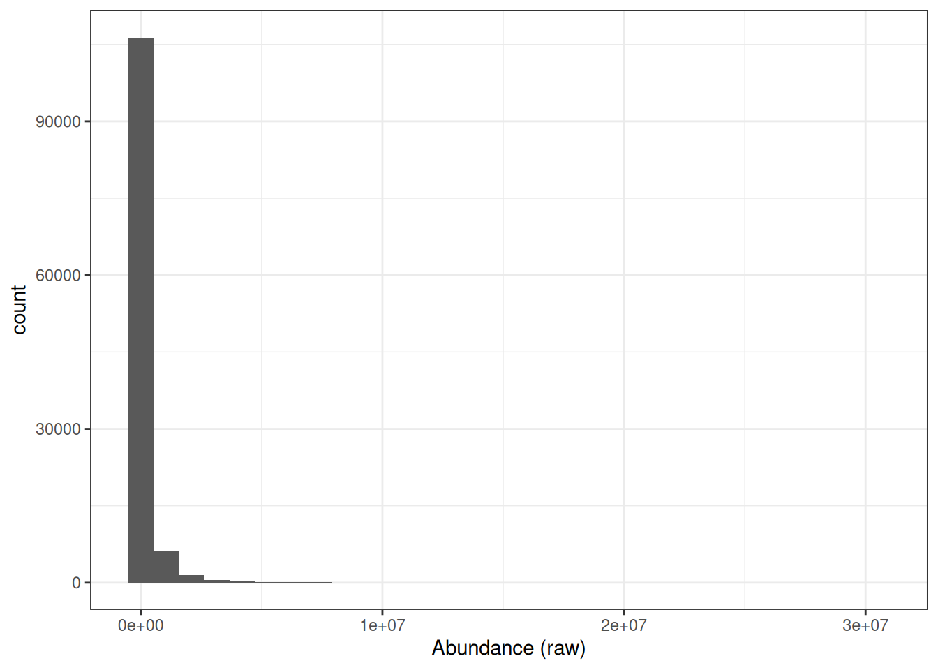
QFeatures objectrobustSummary to summarise precursor-level data to protein-level abundance, including in the presence of missing valuesdiff.median methodHaving filtered our DIA-NN data to retain only high-confidence identifications and removed precursors with excessive missing values, we are now ready to continue processing. In this lesson we will log2 transform the precursor-level data, aggregate to protein-level abundances, and normalise the protein-level data ready for downstream statistical analysis.
If we look at the distribution of raw precursor intensities, we will see that the abundance values are dramatically skewed towards zero.
dia_qf[["precursors_filtered_missing"]] %>%
assay() %>%
longForm() %>%
ggplot(aes(x = value)) +
geom_histogram() +
theme_bw() +
xlab("Abundance (raw)")
This is to be expected since the majority of proteins exist at low abundances within the cell or in serum and only a few are highly abundant. However, raw protein abundances are not normally distributed, which means parametric statistical tests cannot be applied directly.
Why does the skewed distribution matter? Consider a protein with abundance values of 0.25, 1, and 4 across three samples A, B, and C:
By applying a log2 transformation, the values become −2, 0, and +2 — evenly spaced — converting the skewed distribution into a symmetrical, approximately Gaussian distribution suitable for downstream statistical analysis.
Although there is no mathematical reason for applying a log2 transformation rather than using a higher base such as log10, the log2 scale provides an easy visualisation tool. Any protein that halves in abundance between conditions will have a 0.5 fold change, which translates into a log2 fold change of -1. Any protein that doubles in abundance will have a fold change of 2 and a log2 fold change of +1.
Logarithmic transformation should be applied at the appropriate stage of the processing pipeline for the aggregation method being used. Here we apply it before aggregation to protein level, because we use robustSummary for summarisation. robustSummary fits a linear model to the precursor-level data, which assumes approximately Gaussian distributed residuals — a requirement that is only met after log transformation.
We apply a log2 transformation to the filtered precursor data using the logTransform function, which creates a new set in our QFeatures object.
dia_qf <- logTransform(
  dia_qf,
  base = 2,
  i = "precursors_filtered_missing",
  name = "precursors_filtered_missing_log"
)We now aggregate from precursor level to protein level using the aggregateFeatures function. For DIA data with missing values, we use the robustSummary method (Sticker et al. (2020)), which models the log-transformed peptide/precursor-level quantification as being dependent upon the protein-level abundance plus a precursor-level effect. This modelling-based approach can handle missing values without imputation, as it only considers finite data. The only requirement is that a precursor must be quantified in at least two samples.
dia_qf <- aggregateFeatures(
  dia_qf,
  i = "precursors_filtered_missing_log",
  fcol = "Protein.Ids",
  name = "proteins",
  fun = MsCoreUtils::robustSummary,
  maxit = 10000
)
  |
  |                                                                      |   0%
  |
|======================================================================| 100%dia_qfAn instance of class QFeatures (type: bulk) with 5 sets:
[1] precursors: SummarizedExperiment with 4692 rows and 31 columns
[2] precursors_no_cont: SummarizedExperiment with 4417 rows and 31 columns
[3] precursors_filtered_missing: SummarizedExperiment with 4137 rows and 31 columns
[4] precursors_filtered_missing_log: SummarizedExperiment with 4137 rows and 31 columns
[5] proteins: SummarizedExperiment with 368 rows and 31 columns Robust protein identification and quantification depend heavily on the number and quality of peptides detected for each protein. Whilst this workflow does not explicitly demonstrate filtering of single-peptide identifications (“one-hit wonders”), it is considered good practice to assess these carefully during downstream analysis. As a general rule of thumb, the use of at least two unique proteotypic peptides per protein is widely considered best practice. Major peer-reviewed proteomics journals, including Molecular & Cellular Proteomics and Journal of Proteome Research, commonly expect this standard in discovery-based studies to help control false discovery rates (FDR) and improve confidence in protein identification.Although quantification based on a single peptide can be acceptable in targeted workflows such as SRM or PRM, this generally requires that the peptide be well characterized, reproducibly detected, and manually validated. In contrast, discovery-driven proteomics experiments should typically adhere to the two-peptide guideline to maximise confidence, reproducibility, and peer-review acceptance.However, strict enforcement of the two-peptide rule may not always be feasible in studies involving non-model or poorly annotated organisms. In such cases, incomplete genomic or proteomic databases, limited sequence coverage, and high sequence homology can restrict confident identification to a single peptide. Researchers must then apply additional validation strategies, such as manual spectral inspection, orthogonal evidence, or cross-species homology assessment, to support protein identification and quantification.
Level:
Although robustSummary can handle missing values at the precursor level, a protein will still have a missing abundance in any sample where all of its precursors are absent.
To investigate this, we will use the longForm function, which converts a QFeatures set from wide format (proteins × samples) to long format (one row per protein–sample combination). The colvars argument specifies which columns from the colData to carry across.
Run the following code and inspect the output — what does each row represent?
# dia_qf[,,'proteins'] subsets the QFeatures object to the "proteins" set
longForm(dia_qf[,, 'proteins'], colvars = 'group') %>%
  data.frame() %>%
  head()
harmonizing input:
removing 124 sampleMap rows not in names(experiments) assay primary rowname colname value
1 proteins COVID_E1 A0A075B6H7;A0A0C4DH90;A0A0C4DH55;P01624 COVID_E1 19.04836
2 proteins COVID_E1 A0A075B6H9 COVID_E1 12.87679
3 proteins COVID_E1 A0A075B6I0 COVID_E1 14.72490
4 proteins COVID_E1 A0A075B6I9 COVID_E1 13.70752
5 proteins COVID_E1 A0A075B6I9;P04211 COVID_E1 14.86335
6 proteins COVID_E1 A0A075B6J9 COVID_E1 NA
group
1 Covid19
2 Covid19
3 Covid19
4 Covid19
5 Covid19
6 Covid19Now use this long-format data to create a plot showing how many samples each protein is quantified in, broken down by group. Then consider:
robustSummary?sum(is.finite(value)).
Each row in the long-format data represents one protein–sample observation, with value containing the protein abundance and group indicating which experimental group that sample belongs to.
longForm(dia_qf[,, 'proteins'], colvars = 'group') %>%
  data.frame() %>%
  group_by(rowname, group) %>%
  summarise(n_quant = sum(is.finite(value))) %>%
  ggplot(aes(n_quant)) +
  geom_histogram() +
  facet_wrap(~group) +
  theme_classic() +
  labs(x = 'Quantified samples', y = 'Proteins')
harmonizing input:
removing 124 sampleMap rows not in names(experiments)`summarise()` has regrouped the output.
`stat_bin()` using `bins = 30`. Pick better value `binwidth`.
ℹ Summaries were computed grouped by rowname and group.
ℹ Output is grouped by rowname.
ℹ Use `summarise(.groups = "drop_last")` to silence this message.
ℹ Use `summarise(.by = c(rowname, group))` for per-operation grouping
(`?dplyr::dplyr_by`) instead.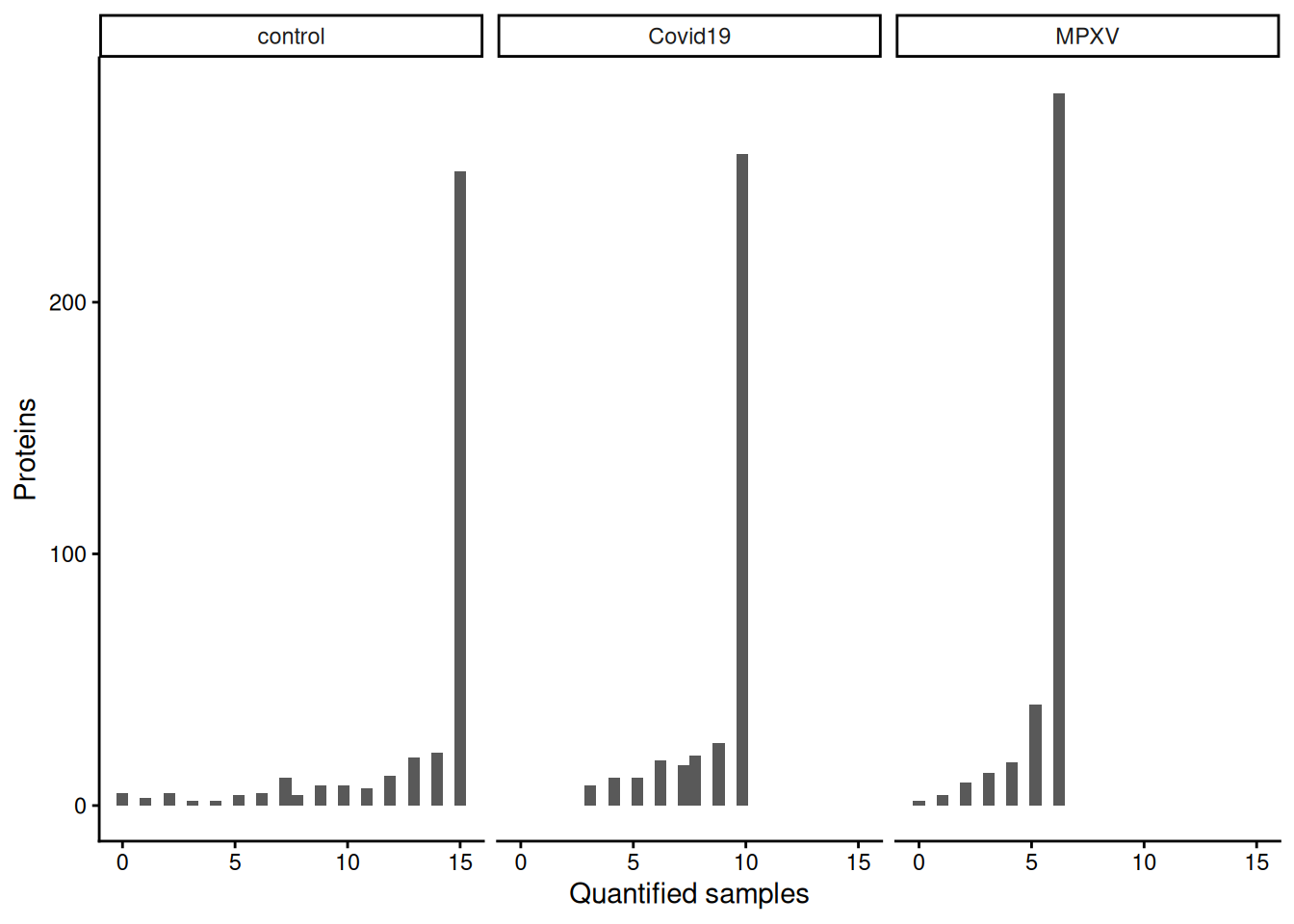
robustSummary estimates protein abundance from whatever precursors are observed in a given sample. If no precursors for a protein are observed in that sample, there is no data from which to estimate abundance, so the protein-level value remains missing regardless of the summarisation method.
Level:
The previous exercise showed how many samples each protein is quantified in, but not which samples. Understanding the pattern of missingness — whether it is random or associated with particular samples or groups — can inform decisions about how to handle missing values downstream.
Use the naniar::gg_miss_upset function to visualise the patterns of missingness in the protein-level data. An upset plot shows which combinations of samples tend to have missing values for the same proteins.
assay(), convert to a data frame, and pass to naniar::gg_miss_upset. Each column (sample) becomes a “set” in the upset plot. Use sets = paste0(colnames(missing_data), "_NA") to control the order of samples, and nintersects to limit the number of intersections shown.
missing_data <- dia_qf[['proteins']] %>% assay() %>% data.frame()

# The sets argument is required to make the keep_order work as intended,
# otherwise the order of the sets is determined by the total number of missing
# values in each set, which is not what we want here. By providing the sets
# argument with the column names of the missing data, we can ensure that the order
# of the sets in the upset plot matches the order of the columns in our data frame.
naniar::gg_miss_upset(
  missing_data,
  sets = paste0(colnames(missing_data), "_NA"),
  keep.order = TRUE,
  nintersects = 50
)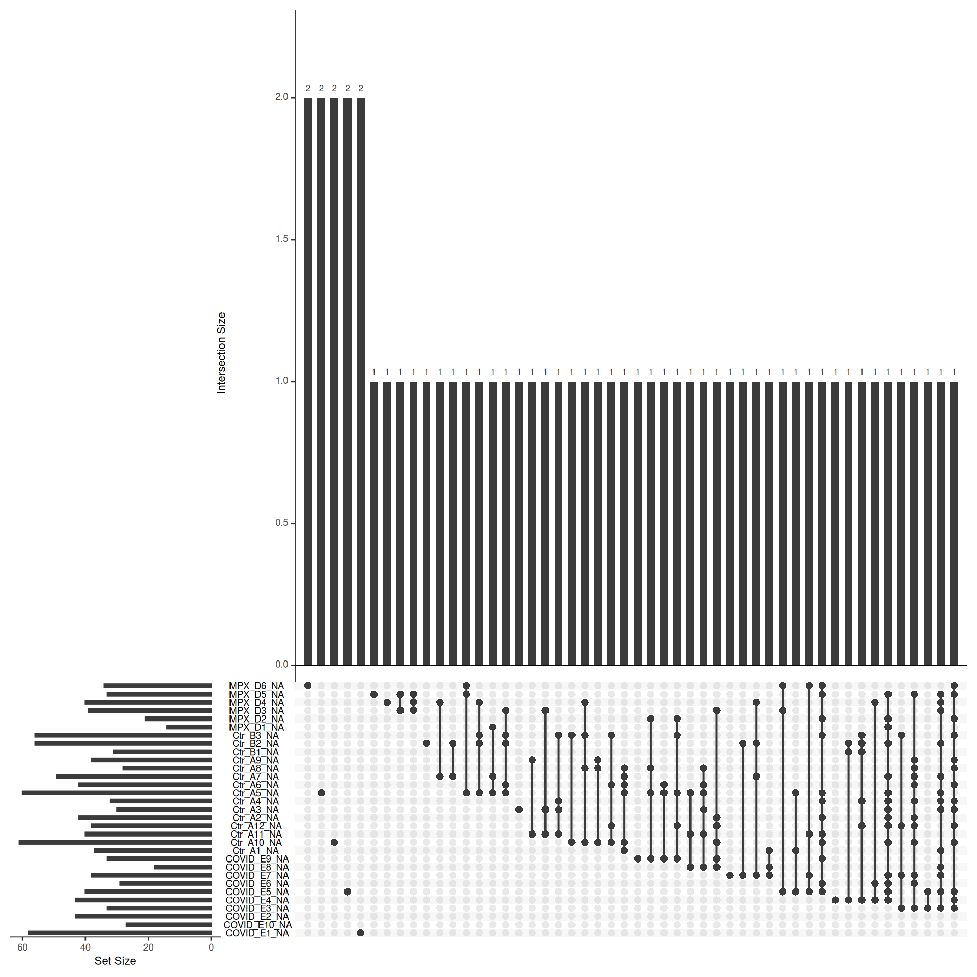
If missing values are clustered within specific groups rather than randomly distributed across samples, this suggests the missingness is intensity-dependent (MNAR) — proteins that are genuinely absent or below the limit of detection in certain conditions. This is biologically informative but has implications for imputation: left-censored methods are more appropriate for MNAR data than methods that assume values are missing at random.
We now have log protein level abundance data to which we could apply a parametric statistical test. However, to perform a statistical test and discover whether any proteins differ in abundance between conditions, we first need to account for non-biological variance that may contribute to any differential abundance. Such variance can arise from experimental error or technical variation, although the latter is much more prominent when dealing with label-free DDA data, compared to TMT DDA or LFQ DIA.
Normalisation is the process by which we account for non-biological variation in protein abundance between samples and attempt to return our quantitative data back to its ‘normal’ condition i.e., representative of how it was in the original biological system. There are various methods that exist to normalise expression proteomics data and it is necessary to consider which of these to apply on a case-by-case basis. Unfortunately, there is not currently a single normalisation method which performs best for all quantitative proteomics datasets.
In QFeatures we can use the normalize function to apply normalisation. To see which methods are supported, type ?normalize to access the function’s help page.
Of the supported methods, median-based methods work well for most quantitative proteomics data. Unlike mean-based methods, median-based normalisation is less sensitive to the extreme values and outliers that are commonly present in proteomics datasets, making it a more robust choice for correcting sample-level systematic differences in loading or ionisation efficiency.
Median-based normalisation works by calculating a single correction factor per sample — the difference between that sample’s median abundance and a reference value — and applying it as a constant shift to every protein in that sample. This means all proteins in a given sample are shifted by the same amount, preserving the relative differences between proteins within each sample while bringing the overall distributions into alignment across samples.
We apply the diff.median method, which shifts each sample’s intensity distribution so that all sample medians match the grand median across all samples.
More sophisticated normalisation approaches may be appropriate depending on the data. For example, the authors of the original study from which this dataset is derived (Wang et al. 2022) used cyclic loess normalisation, available via limma::normalizeCyclicLoess(), which corrects for intensity-dependent biases rather than applying a simple global shift. However, applying it within the QFeatures pipeline requires extracting and replacing the assay matrix manually, and because cyclic loess is sensitive to missing values, additional care is needed — complexity beyond the scope of this course.
dia_qf <- normalize(
  dia_qf,
  i = "proteins",
  name = "norm_proteins",
  method = "diff.median"
)
We can visualise the effect of normalisation by plotting density curves of protein abundance per sample before and after normalisation.
pre_norm <- longForm(dia_qf[,, 'proteins'], colvars = 'group') %>%
  ggplot(aes(x = value, colour = group, group = colname)) +
  geom_density() +
  theme_classic() +
  xlab("log2 (Abundance)") +
  ggtitle('Pre-normalisation')

post_norm <- longForm(dia_qf[,, 'norm_proteins'], colvars = 'group') %>%
  ggplot(aes(x = value, colour = group, group = colname)) +
  geom_density() +
  theme_classic() +
  xlab("log2 (Abundance)") +
  ggtitle('Post-normalisation')

pre_norm + post_norm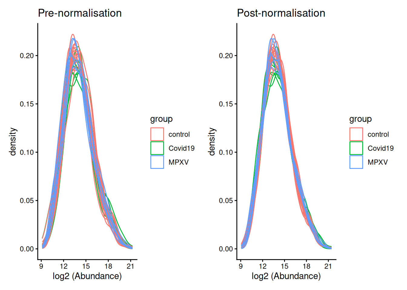
robustSummary is the recommended summarisation method for DIA data, as it can handle missing values at the precursor level without requiring imputationrobustSummary — these should be explored and handled appropriatelydiff.median normalisation corrects for sample-level systematic differences by shifting each sample’s intensity distribution to have the same median