library("arrow")
library("readxl")
library("QFeatures")
library("tidyr")
library("dplyr")
library("ggplot2")
library("patchwork")2 Import and infrastructure
TipLearning Objectives
- Understand the structure of
SummarizedExperimentandQFeaturesobjects and how the two are related - Understand how DIA-NN output data is structured and how it can be imported into R
- Know how to use
readQFeaturesFromDIANNto create aQFeaturesobject from DIA-NN output - Be able to access sample metadata via
colDatain aQFeaturesobject - Be able to explore the data within a
QFeaturesobject usingassay,rowData, andcolData
2.1 The data structure
The raw DIA mass spectrometry data was processed using DIA-NN, which outputs a report file in .parquet format. Unlike a simple abundance matrix, this is a long-format table — each row corresponds to a single precursor–sample combination, rather than one row per precursor across all samples simultaneously. The file contains precursor-level identifications and quantities for every sample, along with quality metrics from the DIA-NN search.
We read this file into R using the read_parquet function from the arrow package.
diann_df <- read_parquet("data/monkeypox_plasma_proteomes.parquet")We can inspect the dimensions and column names to understand what the data contains.
dim(diann_df)[1] 120505 71names(diann_df) [1] "Run.Index" "Run"
[3] "Channel" "Precursor.Id"
[5] "Modified.Sequence" "Stripped.Sequence"
[7] "Precursor.Charge" "Precursor.Lib.Index"
[9] "Decoy" "Proteotypic"
[11] "Precursor.Mz" "Protein.Ids"
[13] "Protein.Group" "Protein.Names"
[15] "Genes" "RT"
[17] "iRT" "Predicted.RT"
[19] "Predicted.iRT" "IM"
[21] "iIM" "Predicted.IM"
[23] "Predicted.iIM" "Precursor.Quantity"
[25] "Precursor.Normalised" "Ms1.Area"
[27] "Ms1.Normalised" "Ms1.Apex.Area"
[29] "Ms1.Apex.Mz.Delta" "Normalisation.Factor"
[31] "Quantity.Quality" "Empirical.Quality"
[33] "Normalisation.Noise" "Ms1.Profile.Corr"
[35] "Evidence" "Mass.Evidence"
[37] "Channel.Evidence" "Ms1.Total.Signal.Before"
[39] "Ms1.Total.Signal.After" "RT.Start"
[41] "RT.Stop" "FWHM"
[43] "PG.TopN" "PG.MaxLFQ"
[45] "Genes.TopN" "Genes.MaxLFQ"
[47] "Genes.MaxLFQ.Unique" "PG.MaxLFQ.Quality"
[49] "Genes.MaxLFQ.Quality" "Genes.MaxLFQ.Unique.Quality"
[51] "Q.Value" "PEP"
[53] "Global.Q.Value" "Lib.Q.Value"
[55] "Peptidoform.Q.Value" "Global.Peptidoform.Q.Value"
[57] "Lib.Peptidoform.Q.Value" "PTM.Site.Confidence"
[59] "Site.Occupancy.Probabilities" "Protein.Sites"
[61] "Lib.PTM.Site.Confidence" "Translated.Q.Value"
[63] "Channel.Q.Value" "PG.Q.Value"
[65] "PG.PEP" "GG.Q.Value"
[67] "Protein.Q.Value" "Global.PG.Q.Value"
[69] "Lib.PG.Q.Value" "Best.Fr.Mz"
[71] "Best.Fr.Mz.Delta" The key columns we will use in our analysis are:
Precursor.Id: a unique identifier for each precursor — typically the modified peptide sequence and charge state (e.g."PEPTM[ox]IDEQ..2")Protein.Group: the canonical protein group identifier used for aggregation to protein level. Proteins that cannot be distinguished from each other based on proteotypic peptides detected in the data are grouped together under one Protein Group.Protein.Ids: the UniProt accession(s) of the protein(s) to which the precursor is assignedGenes: the gene symbol(s) associated with the identified proteinsRun: the identifier for the sample run — one value per LC-MS sample injectionPrecursor.Quantity: the quantified abundance of the precursor in that runQ.Value: the precursor-level Q-value, representing the estimated false discovery rate at the precursor level; lower values indicate more confident identificationsLib.Q.Value: the library-level Q-value — the confidence that the precursor was matched to the correct entry in the spectral libraryProtein.Q.Value: the protein-level Q-value, representing the estimated FDR at the protein level
The report also contains chromatographic quality metrics per precursor per run. For example:
FWHM: Full-Width at Half Maximum of the chromatographic peak, a measure of peak shape quality — narrow, symmetrical peaks are preferred
We will use these Q-value columns and quality metrics to filter the data in the next lesson.
We will be using the QFeatures Bioconductor package to import, store, and manipulate our data. Before we import the data it is first necessary to understand the structure of a QFeatures object and its underlying SummarizedExperiment objects.
2.2 The structure of a SummarizedExperiment
To simplify the storage of quantitative proteomics data we can store the data as a SummarizedExperiment object (as shown in Figure 10.1). SummarizedExperiment objects can be conceptualised as data containers made up of three different parts:
The
assay- a matrix which contains the quantitative data from a proteomics experiment. Each row represents a feature (a precursor, peptide or protein) and each column contains the quantitative data (measurements) from one experimental sample.The
rowData- a table (data frame) which contains all remaining information associated with each feature (i.e. every column from your search output that was not a quantification column). Rows represent features but columns inform about different attributes of the feature (e.g., its sequence, name, modifications).The
colData- a table (data frame) to store sample metadata that would not appear in the output of your search software. This could be, for example, the condition, replicate, or batch each sample belongs to. Again, this information is stored in a matrix-like data structure.
Finally, there is also an additional container called metadata which is a place for users to store experimental metadata, such as which instrument the samples were run on or the date of data acquisition. We will focus on populating and understanding the three main containers above.
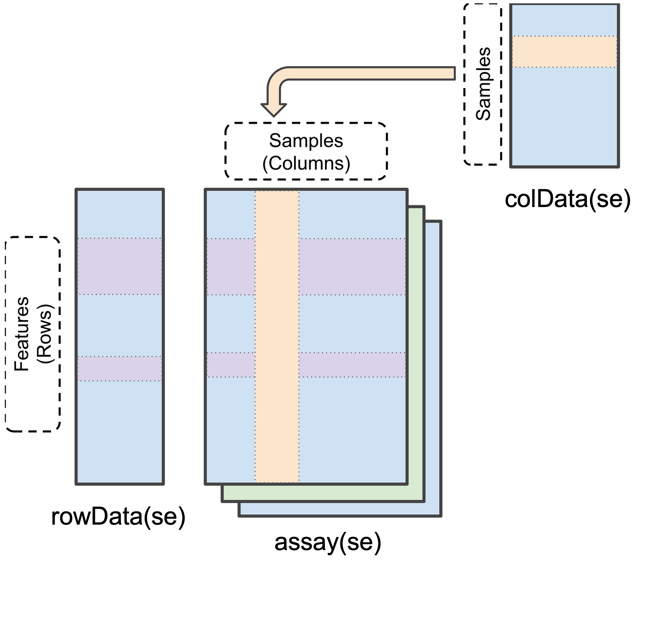
SummarizedExperiment object in R (modified from the SummarizedExperiment package)
Data stored in these three main areas can be easily accessed using the assay(), rowData() and colData() functions, as we will see later.
2.3 The structure of a QFeatures object
Whilst a SummarizedExperiment is able to neatly store quantitative proteomics data at a single data level (i.e., precursor, peptide or protein), a typical data analysis workflow requires us to look across multiple levels. For example, it is common to start an analysis at a lower data level and then aggregate upward towards a final protein-level dataset. Doing this allows for greater flexibility and understanding of the processes required to clean and aggregate the data.
A QFeatures object is essentially a list of SummarizedExperiment objects. However, the main benefit of using a QFeatures object over storing each data level as an independent SummarizedExperiment is that the QFeatures infrastructure maintains explicit links between the SummarizedExperiments that it stores. This allows for maximum traceability when processing data across multiple levels — for example, tracking which precursors or peptides contribute to each protein (Figure 10.2, modified from the QFeatures vignette with permission).
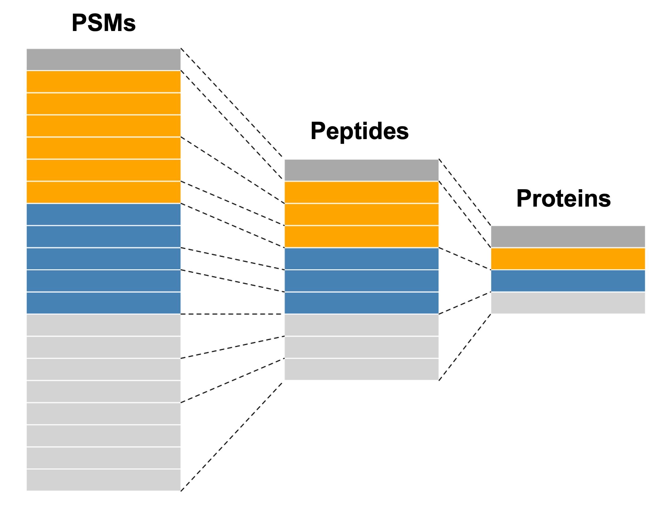
QFeatures object.
NoteQFeatures nomenclature
When talking about a QFeatures object, each dataset (individual SummarizedExperiment) can be referred to as a set (short for dataset). Previously, each dataset was referred to as an experimental assay, and some older resources may still use this term. However, the experimental assay should not be confused with the quantitative matrix section of a SummarizedExperiment, which is called the assay data.
In order to generate the explicit links between data levels, we need to import the lowest desired data level into a QFeatures object and aggregate upwards within the QFeatures infrastructure using the aggregateFeatures function. If two SummarizedExperiments are generated separately and then added into the same QFeatures object, there will not automatically be links between them. In this case, if links are required, we can manually add them using the addAssayLink() function.
The best way to get our head around the QFeatures infrastructure is to import our data into a QFeatures object and start exploring.
2.4 Importing sample metadata
Sample metadata is information related to each sample that helps us interpret, organise and analyse our proteomics data. This data is something you must create yourself, related to your experiment. You can use a spreadsheet program such as Excel, or it can be coded in R directly.
Here, we have created a sample metadata file in Excel. This file is called monkeypox_metadata.xlsx. It provides information about each sample, including which group (MPXV, COVID-19, or Control) each run belongs to. We use the read_excel function from the readxl package to import the data into R.
sample_metadata <- read_excel("data/monkeypox_metadata.xlsx")
print(sample_metadata)
# A tibble: 31 × 5
sample_id runCol group sex age.group
<chr> <chr> <chr> <chr> <chr>
1 20220624_Z1_ZW_001_30-0066_Ctr-A1_heat_DIA Ctr_A1 control m 21-30
2 20220624_Z1_ZW_001_30-0066_Ctr-A10_heat_DIA Ctr_A10 control m 31-40
3 20220624_Z1_ZW_001_30-0066_Ctr-A11_heat_DIA Ctr_A11 control m 31-40
4 20220624_Z1_ZW_001_30-0066_Ctr-A12_heat_DIA Ctr_A12 control m 41-50
5 20220624_Z1_ZW_001_30-0066_Ctr-A2_heat_DIA Ctr_A2 control m 21-30
6 20220624_Z1_ZW_001_30-0066_Ctr-A3_heat_DIA Ctr_A3 control m 21-30
7 20220624_Z1_ZW_001_30-0066_Ctr-A4_heat_DIA Ctr_A4 control m 21-30
8 20220624_Z1_ZW_001_30-0066_Ctr-A5_heat_DIA Ctr_A5 control m 21-30
9 20220624_Z1_ZW_001_30-0066_Ctr-A6_heat_DIA Ctr_A6 control m 21-30
10 20220624_Z1_ZW_001_30-0066_Ctr-A7_heat_DIA Ctr_A7 control m 21-30
# ℹ 21 more rowsThere are several columns in this file including the sample_id which is the name of the sample as well as the group, sex and age group. We have also created a column called runCol which is a concise, human-readable label for each sample which we add to our diann_df to in the next section to use in our analysis.
NoteThe pipe operator
In this course we will frequently use the pipe operator (%>%) from the dplyr package and tidyverse. The pipe passes the output of one function directly as the input to the next, allowing you to chain together multiple operations in a linear, readable way — rather than nesting function calls or creating many intermediate variables. For more information see Hadley Wickham’s Tidyverse at https://www.tidyverse.org.
2.4.1 Cleaning run names
In DIA-NN the names in the Run column often inherit the full raw file path pasting together the name of the .wiff2 folder and the .wiff.scan files (.wiff files are raw data formats generated by SCIEX mass spectrometers containing unprocessed metadata and scan data from LM-MS/MS runs). We need to clean up these run names so that they match the sample_id field in our metadata.
# Clean Run names
diann_df[, "Run"] %>%
  unique() %>%
  head(2)
# A tibble: 2 × 1
Run
<chr>
1 20220624_Z1_ZW_001_30-0066_COVID-E9_heat_DIA.wiff2-20220624_Z1_ZW_001_30-0066…
2 20220624_Z1_ZW_001_30-0066_MPX-D2_heat_DIA.wiff2-20220624_Z1_ZW_001_30-0066_M…# DIANN has pasted the name of the .wiff2 folder as well as the .wiff.scan
# files together. So we need to clean up the Run names so that they match
# the metadata `sample_id` field.
diann_df <- diann_df %>%
mutate(Run = sub('\\..*', '', Run))
# Check we have cleaned the Run names
diann_df[, "Run"] %>%
unique() %>%
head(2)# A tibble: 2 × 1
Run
<chr>
1 20220624_Z1_ZW_001_30-0066_COVID-E9_heat_DIA
2 20220624_Z1_ZW_001_30-0066_MPX-D2_heat_DIA In the following code chunk we add a new column called runCol to the diann_df data. This column will serve as a link between the metadata and the diann_df proteomics data as well as being useful for visualisation and annotating our data at a later stage in the analysis.
diann_df <- diann_df %>%
  merge(
    sample_metadata[, c("sample_id", "runCol")],
    by.x = "Run",
    by.y = "sample_id"
  )
If we look at the column dimensions and names of the diann_df we now see the runCol column has been added.
dim(diann_df)[1] 120505 72names(diann_df) [1] "Run" "Run.Index"
[3] "Channel" "Precursor.Id"
[5] "Modified.Sequence" "Stripped.Sequence"
[7] "Precursor.Charge" "Precursor.Lib.Index"
[9] "Decoy" "Proteotypic"
[11] "Precursor.Mz" "Protein.Ids"
[13] "Protein.Group" "Protein.Names"
[15] "Genes" "RT"
[17] "iRT" "Predicted.RT"
[19] "Predicted.iRT" "IM"
[21] "iIM" "Predicted.IM"
[23] "Predicted.iIM" "Precursor.Quantity"
[25] "Precursor.Normalised" "Ms1.Area"
[27] "Ms1.Normalised" "Ms1.Apex.Area"
[29] "Ms1.Apex.Mz.Delta" "Normalisation.Factor"
[31] "Quantity.Quality" "Empirical.Quality"
[33] "Normalisation.Noise" "Ms1.Profile.Corr"
[35] "Evidence" "Mass.Evidence"
[37] "Channel.Evidence" "Ms1.Total.Signal.Before"
[39] "Ms1.Total.Signal.After" "RT.Start"
[41] "RT.Stop" "FWHM"
[43] "PG.TopN" "PG.MaxLFQ"
[45] "Genes.TopN" "Genes.MaxLFQ"
[47] "Genes.MaxLFQ.Unique" "PG.MaxLFQ.Quality"
[49] "Genes.MaxLFQ.Quality" "Genes.MaxLFQ.Unique.Quality"
[51] "Q.Value" "PEP"
[53] "Global.Q.Value" "Lib.Q.Value"
[55] "Peptidoform.Q.Value" "Global.Peptidoform.Q.Value"
[57] "Lib.Peptidoform.Q.Value" "PTM.Site.Confidence"
[59] "Site.Occupancy.Probabilities" "Protein.Sites"
[61] "Lib.PTM.Site.Confidence" "Translated.Q.Value"
[63] "Channel.Q.Value" "PG.Q.Value"
[65] "PG.PEP" "GG.Q.Value"
[67] "Protein.Q.Value" "Global.PG.Q.Value"
[69] "Lib.PG.Q.Value" "Best.Fr.Mz"
[71] "Best.Fr.Mz.Delta" "runCol" head(diann_df) Run Run.Index Channel
1 20220624_Z1_ZW_001_30-0066_COVID-E1_heat_DIA 0
2 20220624_Z1_ZW_001_30-0066_COVID-E1_heat_DIA 0
3 20220624_Z1_ZW_001_30-0066_COVID-E1_heat_DIA 0
4 20220624_Z1_ZW_001_30-0066_COVID-E1_heat_DIA 0
5 20220624_Z1_ZW_001_30-0066_COVID-E1_heat_DIA 0
6 20220624_Z1_ZW_001_30-0066_COVID-E1_heat_DIA 0
Precursor.Id Modified.Sequence Stripped.Sequence Precursor.Charge
1 FEVQVTVPK2 FEVQVTVPK FEVQVTVPK 2
2 MTSNFPVDLSDYPK2 MTSNFPVDLSDYPK MTSNFPVDLSDYPK 2
3 IEIPLPFGGK2 IEIPLPFGGK IEIPLPFGGK 2
4 YPLYVLK2 YPLYVLK YPLYVLK 2
5 SGSLPDDVLLHFAGAGK2 SGSLPDDVLLHFAGAGK SGSLPDDVLLHFAGAGK 2
6 DQEVLLQTFLDDASPGDK3 DQEVLLQTFLDDASPGDK DQEVLLQTFLDDASPGDK 3
Precursor.Lib.Index Decoy Proteotypic Precursor.Mz Protein.Ids Protein.Group
1 1172 0 1 523.7977 P01023 P01023
2 2731 0 1 807.3795 P04114 P04114
3 1852 0 1 535.8159 P04114 P04114
4 4673 0 1 448.2680 Q96IY4 Q96IY4
5 3469 0 1 842.4387 Cont_Q1WEI2 Cont_Q1WEI2
6 655 0 1 664.3250 P04114 P04114
Protein.Names Genes RT iRT Predicted.RT Predicted.iRT IM iIM
1 A2MG_HUMAN A2M 11.96337 36.66281 11.97756 36.64785 0 0
2 APOB_HUMAN APOB 15.01260 59.30375 15.01478 59.31506 0 0
3 APOB_HUMAN APOB 17.63608 81.23773 17.68024 81.04679 0 0
4 CBPB2_HUMAN CPB2 13.32482 46.44064 13.32074 46.62988 0 0
5 Q1WEI2_PSEAI prpL 16.89660 73.70802 16.92624 73.39013 0 0
6 APOB_HUMAN APOB 19.05460 95.88051 19.04843 96.30724 0 0
Predicted.IM Predicted.iIM Precursor.Quantity Precursor.Normalised Ms1.Area
1 0 0 1653567.750 1421358.375 966520
2 0 0 90330.430 79665.422 75105
3 0 0 261497.078 210192.125 82467
4 0 0 28442.559 24802.588 12189
5 0 0 6343.696 6343.696 6940
6 0 0 4285.400 3333.609 1919
Ms1.Normalised Ms1.Apex.Area Ms1.Apex.Mz.Delta Normalisation.Factor
1 830792.312 941713 -0.0018310547 0.8595707
2 66237.609 50544 -0.0004882812 0.8819334
3 66287.211 79796 -0.0010375977 0.8038030
4 10629.098 12189 -0.0047912598 0.8720238
5 6940.000 2081 -0.0009155273 0.8904678
6 1492.789 1738 0.0016479492 0.7778993
Quantity.Quality Empirical.Quality Normalisation.Noise Ms1.Profile.Corr
1 0.9687976 0.9761357 -0.12298305 0.9922303557
2 0.9152004 0.9340791 -0.05845552 0.9640983343
3 0.9584711 0.9566879 0.02224668 0.9803985953
4 0.9096999 0.9261814 -0.09447396 0.6928093433
5 0.8393960 0.8298689 -0.18295603 0.0007709147
6 0.8870641 0.8874608 0.06335557 0.7479561567
Evidence Mass.Evidence Channel.Evidence Ms1.Total.Signal.Before
1 6.766142 4.9693527 0.9730694 11857848
2 5.486723 1.8805708 0.8883088 11073541
3 6.613742 1.9588757 0.9622874 8957568
4 4.688177 2.9466224 0.9544354 10839082
5 2.930316 0.4402728 0.2534788 13242398
6 4.777808 0.0000000 0.7815723 5950656
Ms1.Total.Signal.After RT.Start RT.Stop FWHM PG.TopN PG.MaxLFQ
1 10346640 11.84572 12.05762 0.09868256 0 2093697.62
2 13289225 14.84780 15.17732 0.21342939 0 329647.25
3 10203101 17.54195 17.73022 0.08662415 0 329647.25
4 10765211 13.23067 13.41895 0.07194020 0 21966.11
5 14529216 16.73183 17.06133 0.05618586 0 491769.47
6 4521497 18.98402 19.12527 0.04003905 0 329647.25
Genes.TopN Genes.MaxLFQ Genes.MaxLFQ.Unique PG.MaxLFQ.Quality
1 0 2093697.62 1581720.50 0.9925535
2 0 329647.25 329647.25 0.9905457
3 0 329647.25 329647.25 0.9905457
4 0 21966.11 21966.11 0.9400502
5 0 0.00 0.00 0.9817796
6 0 329647.25 329647.25 0.9905457
Genes.MaxLFQ.Quality Genes.MaxLFQ.Unique.Quality Q.Value PEP
1 0.9925535 0.9920511 1.565558e-03 0.0040921429
2 0.9905457 0.9905457 5.040323e-06 0.0000100781
3 0.9905457 0.9905457 5.040323e-06 0.0000100781
4 0.9400502 0.9400502 5.040323e-06 0.0000100781
5 0.0000000 0.0000000 3.268945e-03 0.0122970762
6 0.9905457 0.9905457 5.040323e-06 0.0000100781
Global.Q.Value Lib.Q.Value Peptidoform.Q.Value Global.Peptidoform.Q.Value
1 3.155570e-06 3.412969e-06 0 2.423655e-06
2 3.155570e-06 3.412969e-06 0 2.423655e-06
3 3.155570e-06 3.412969e-06 0 2.423655e-06
4 3.155570e-06 3.507541e-06 0 2.423655e-06
5 3.272251e-06 4.405286e-06 0 2.513273e-06
6 3.155570e-06 3.523608e-06 0 2.423655e-06
Lib.Peptidoform.Q.Value PTM.Site.Confidence Site.Occupancy.Probabilities
1 2.032158e-06 1
2 2.032158e-06 1
3 2.032158e-06 1
4 2.088469e-06 1
5 2.623006e-06 1
6 2.098035e-06 1
Protein.Sites Lib.PTM.Site.Confidence Translated.Q.Value Channel.Q.Value
1 1 0 0
2 1 0 0
3 1 0 0
4 1 0 0
5 1 0 0
6 1 0 0
PG.Q.Value PG.PEP GG.Q.Value Protein.Q.Value Global.PG.Q.Value
1 0.004016064 0.01531236 0.00406504 0.004444445 0.002747253
2 0.004016064 0.01531236 0.00406504 0.004444445 0.002747253
3 0.004016064 0.01531236 0.00406504 0.004444445 0.002747253
4 0.004016064 0.01531236 0.00406504 0.004444445 0.002747253
5 0.004016064 0.01531236 0.00406504 0.004444445 0.002747253
6 0.004016064 0.01531236 0.00406504 0.004444445 0.002747253
Lib.PG.Q.Value Best.Fr.Mz Best.Fr.Mz.Delta runCol
1 0.002525253 376.1867 -3.051758e-03 COVID_E1
2 0.002525253 1033.5200 -2.807617e-03 COVID_E1
3 0.002525253 505.2769 -3.051758e-05 COVID_E1
4 0.002525253 366.7364 -2.014160e-03 COVID_E1
5 0.002525253 232.0928 -2.883911e-03 COVID_E1
6 0.002525253 373.1354 -2.044678e-03 COVID_E12.5 Reading into a QFeatures object
We use the readQFeaturesFromDIANN function to import the cleaned DIA-NN data into a QFeatures object. This function creates one SummarizedExperiment per run, with each set containing the precursor-level quantification data for that run. The runCol argument specifies which column in the input data frame identifies the run.
dia_qf <-
  readQFeaturesFromDIANN(
    diann_df,
    quantCols = "Precursor.Quantity",
    fnames = "Precursor.Id",
    runCol = "runCol",
    colData = sample_metadata
  )
Checking arguments.Loading data as a 'SummarizedExperiment' object.Splitting data in runs.
  |
  |                                                                      |   0%
  |
  |==                                                                    |   3%
  |
  |=====                                                                 |   6%
  |
  |=======                                                               |  10%
  |
  |=========                                                             |  13%
  |
  |===========                                                           |  16%
  |
  |==============                                                        |  19%
  |
  |================                                                      |  23%
  |
  |==================                                                    |  26%
  |
  |====================                                                  |  29%
  |
  |=======================                                               |  32%
  |
  |=========================                                             |  35%
  |
  |===========================                                           |  39%
  |
  |=============================                                         |  42%
  |
  |================================                                      |  45%
  |
  |==================================                                    |  48%
  |
  |====================================                                  |  52%
  |
  |======================================                                |  55%
  |
  |=========================================                             |  58%
  |
  |===========================================                           |  61%
  |
  |=============================================                         |  65%
  |
  |===============================================                       |  68%
  |
  |==================================================                    |  71%
  |
  |====================================================                  |  74%
  |
  |======================================================                |  77%
  |
  |========================================================              |  81%
  |
  |===========================================================           |  84%
  |
  |=============================================================         |  87%
  |
  |===============================================================       |  90%
  |
  |=================================================================     |  94%
  |
  |====================================================================  |  97%
  |
  |======================================================================| 100%
Formatting sample annotations (colData).Formatting data as a 'QFeatures' object.Setting assay rownames.2.6 Exploring the data
When we inspect our QFeatures object, we see that it contains 31 sets, each corresponding to a different sample run. Each set contains the precursor-level quantification data for that run, with feature names given by the Precursor.Id column from the original DIA-NN output.
dia_qfAn instance of class QFeatures (type: bulk) with 31 sets:
[1] COVID_E1: SummarizedExperiment with 3834 rows and 1 columns
[2] COVID_E10: SummarizedExperiment with 3914 rows and 1 columns
[3] COVID_E2: SummarizedExperiment with 4016 rows and 1 columns
...
[29] MPX_D4: SummarizedExperiment with 3950 rows and 1 columns
[30] MPX_D5: SummarizedExperiment with 4043 rows and 1 columns
[31] MPX_D6: SummarizedExperiment with 3861 rows and 1 columns By default if a QFeatures object has more than 6 samples, only the first three and last three sample summaries are printed to the screen. To see all samples and their respective data summary, we can use the experiments function.
experiments(dia_qf)ExperimentList class object of length 31:
[1] COVID_E1: SummarizedExperiment with 3834 rows and 1 columns
[2] COVID_E10: SummarizedExperiment with 3914 rows and 1 columns
[3] COVID_E2: SummarizedExperiment with 4016 rows and 1 columns
[4] COVID_E3: SummarizedExperiment with 4028 rows and 1 columns
[5] COVID_E4: SummarizedExperiment with 3978 rows and 1 columns
[6] COVID_E5: SummarizedExperiment with 3662 rows and 1 columns
[7] COVID_E6: SummarizedExperiment with 3915 rows and 1 columns
[8] COVID_E7: SummarizedExperiment with 3950 rows and 1 columns
[9] COVID_E8: SummarizedExperiment with 3882 rows and 1 columns
[10] COVID_E9: SummarizedExperiment with 3906 rows and 1 columns
[11] Ctr_A1: SummarizedExperiment with 3878 rows and 1 columns
[12] Ctr_A10: SummarizedExperiment with 3894 rows and 1 columns
[13] Ctr_A11: SummarizedExperiment with 3800 rows and 1 columns
[14] Ctr_A12: SummarizedExperiment with 3876 rows and 1 columns
[15] Ctr_A2: SummarizedExperiment with 3864 rows and 1 columns
[16] Ctr_A3: SummarizedExperiment with 4105 rows and 1 columns
[17] Ctr_A4: SummarizedExperiment with 3823 rows and 1 columns
[18] Ctr_A5: SummarizedExperiment with 3759 rows and 1 columns
[19] Ctr_A6: SummarizedExperiment with 3903 rows and 1 columns
[20] Ctr_A7: SummarizedExperiment with 3774 rows and 1 columns
[21] Ctr_A8: SummarizedExperiment with 3936 rows and 1 columns
[22] Ctr_A9: SummarizedExperiment with 3856 rows and 1 columns
[23] Ctr_B1: SummarizedExperiment with 3936 rows and 1 columns
[24] Ctr_B2: SummarizedExperiment with 3819 rows and 1 columns
[25] Ctr_B3: SummarizedExperiment with 3788 rows and 1 columns
[26] MPX_D1: SummarizedExperiment with 3845 rows and 1 columns
[27] MPX_D2: SummarizedExperiment with 3858 rows and 1 columns
[28] MPX_D3: SummarizedExperiment with 3852 rows and 1 columns
[29] MPX_D4: SummarizedExperiment with 3950 rows and 1 columns
[30] MPX_D5: SummarizedExperiment with 4043 rows and 1 columns
[31] MPX_D6: SummarizedExperiment with 3861 rows and 1 columnsWe can quickly see how many precursors were measure per sample for example, we see for the first sample called COVID_E1 there are 3834 precursors.
We can access individual samples (sets, or SummarizedExperiments) using standard double bracket nomenclature (this is how you would normally access items of a list in R). As with all indexing we can use the list position or dataset name.
dia_qf[[1]]class: SummarizedExperiment
dim: 3834 1
metadata(0):
assays(1): ''
rownames(3834): FEVQVTVPK2 MTSNFPVDLSDYPK2 ... VLTPPMGTVMDVLK2
LSHNAIASLRPR3
rowData names(71): Run Run.Index ... Best.Fr.Mz.Delta runCol
colnames(1): COVID_E1
colData names(0):Is the same as,
dia_qf[["COVID_E1"]]class: SummarizedExperiment
dim: 3834 1
metadata(0):
assays(1): ''
rownames(3834): FEVQVTVPK2 MTSNFPVDLSDYPK2 ... VLTPPMGTVMDVLK2
LSHNAIASLRPR3
rowData names(71): Run Run.Index ... Best.Fr.Mz.Delta runCol
colnames(1): COVID_E1
colData names(0):The quantitation data for each sample is store in the assay container and can be extracted using the assay function.
assay(dia_qf[[1]]) %>%
  head()
COVID_E1
FEVQVTVPK2 1653567.750
MTSNFPVDLSDYPK2 90330.430
IEIPLPFGGK2 261497.078
YPLYVLK2 28442.559
SGSLPDDVLLHFAGAGK2 6343.696
DQEVLLQTFLDDASPGDK3 4285.400Discussion
Why does readQFeaturesFromDIANN create one SummarizedExperiment per run, rather than a single combined set across all runs from the outset?
2.6.1 How many precursors per sample?
Each sample will have a different number of precursors identified and quantified. We can explore this by inspecting the number of rows in each per-sample set, which corresponds to the number of precursors quantified in that sample.
ExerciseExercise 1 - Challenge: Precursors per sample
Level:
Find a function to determine how many precursors are quantified in each sample. Use it to plot a histogram of precursor counts across samples.
Create a bar plot showing the number of precursors identified in each sample, coloured by group. Based on your plot:
- Which group tends to have the most precursors identified?
- Is there any sample that looks like an outlier?
Hint
Browse theQFeatures documentation with ?QFeatures to find a suitable function for obtaining per-sample feature counts.
AnswerAnswer
Task 1
hist(nrows(dia_qf), xlab = "Precursors", main = "Precursor counts per sample")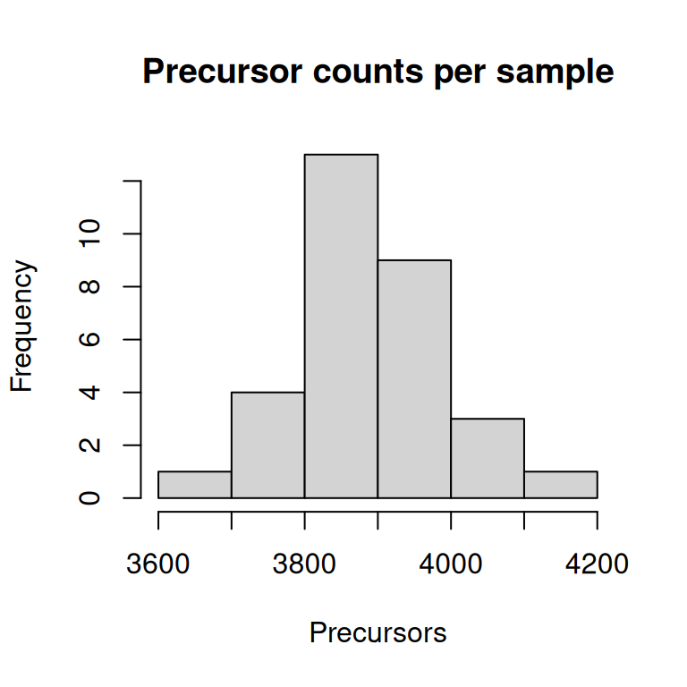
Task 2
data.frame(
  n_precursors = nrows(dia_qf),
  sample = names(nrows(dia_qf))
) %>%
  merge(data.frame(colData(dia_qf)), by.x = "sample", by.y = "runCol") %>%
  ggplot(aes(x = sample, y = n_precursors, fill = group)) +
  geom_bar(stat = "identity") +
  labs(x = "Sample", y = "Number of precursors") +
  coord_flip() +
  theme_classic()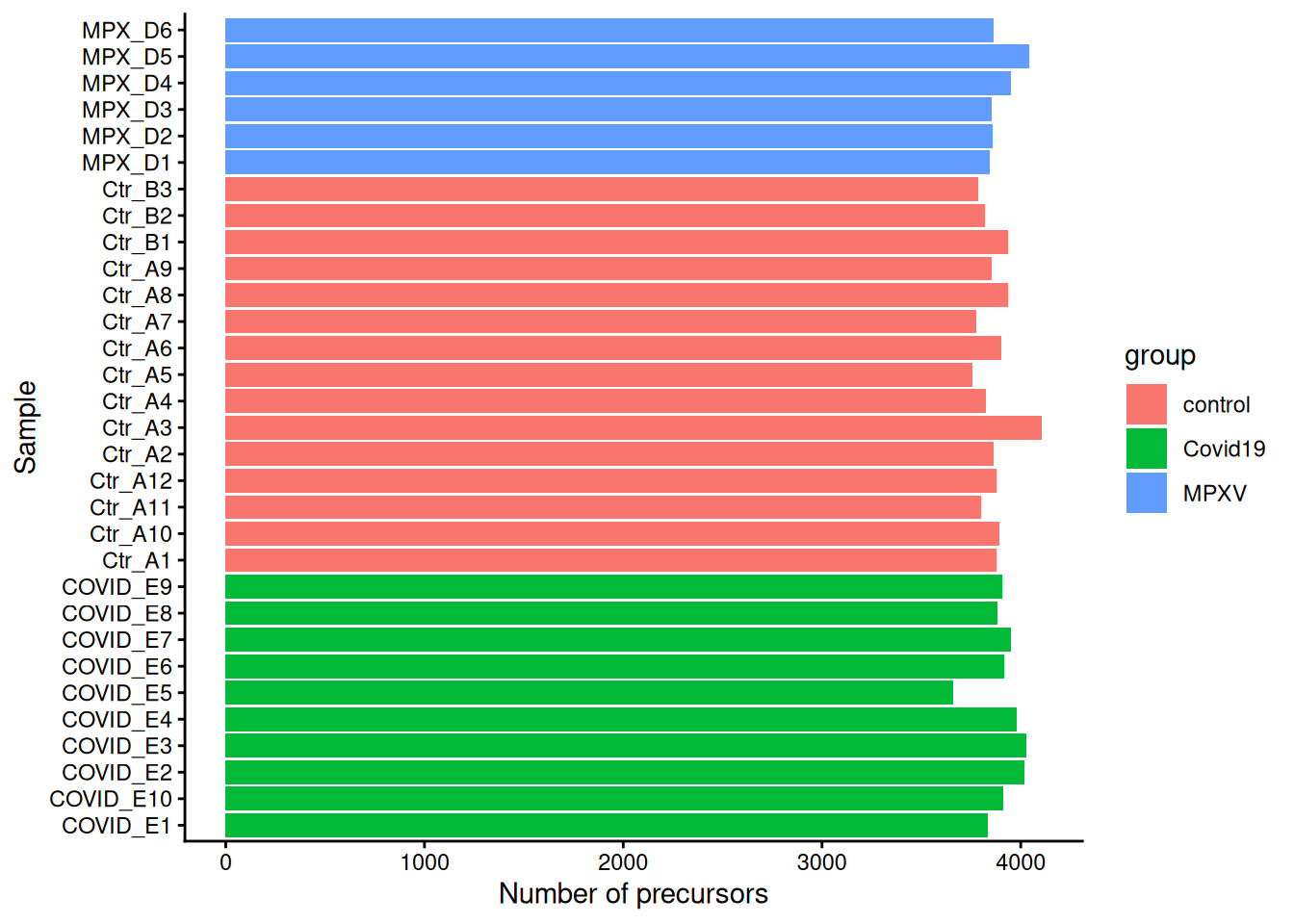
2.6.2 Exploring the row data
The rowData of each per-sample SummarizedExperiment contains quality metrics from DIA-NN. This information can be accessed on a sample by sample level by using the rowData function.
rowData(dia_qf[[1]]) %>%
  head(2)
DataFrame with 2 rows and 71 columns
Run Run.Index Channel Precursor.Id
<character> <integer> <character> <character>
FEVQVTVPK2 20220624_Z... 0 FEVQVTVPK2
MTSNFPVDLSDYPK2 20220624_Z... 0 MTSNFPVDLS...
Modified.Sequence Stripped.Sequence Precursor.Charge
<character> <character> <integer>
FEVQVTVPK2 FEVQVTVPK FEVQVTVPK 2
MTSNFPVDLSDYPK2 MTSNFPVDLS... MTSNFPVDLS... 2
Precursor.Lib.Index Decoy Proteotypic Precursor.Mz
<integer> <integer> <integer> <numeric>
FEVQVTVPK2 1172 0 1 523.798
MTSNFPVDLSDYPK2 2731 0 1 807.379
Protein.Ids Protein.Group Protein.Names Genes RT
<character> <character> <character> <character> <numeric>
FEVQVTVPK2 P01023 P01023 A2MG_HUMAN A2M 11.9634
MTSNFPVDLSDYPK2 P04114 P04114 APOB_HUMAN APOB 15.0126
iRT Predicted.RT Predicted.iRT IM iIM
<numeric> <numeric> <numeric> <numeric> <numeric>
FEVQVTVPK2 36.6628 11.9776 36.6478 0 0
MTSNFPVDLSDYPK2 59.3037 15.0148 59.3151 0 0
Predicted.IM Predicted.iIM Precursor.Normalised Ms1.Area
<numeric> <numeric> <numeric> <numeric>
FEVQVTVPK2 0 0 1421358.4 966520
MTSNFPVDLSDYPK2 0 0 79665.4 75105
Ms1.Normalised Ms1.Apex.Area Ms1.Apex.Mz.Delta
<numeric> <numeric> <numeric>
FEVQVTVPK2 830792.3 941713 -0.001831055
MTSNFPVDLSDYPK2 66237.6 50544 -0.000488281
Normalisation.Factor Quantity.Quality Empirical.Quality
<numeric> <numeric> <numeric>
FEVQVTVPK2 0.859571 0.968798 0.976136
MTSNFPVDLSDYPK2 0.881933 0.915200 0.934079
Normalisation.Noise Ms1.Profile.Corr Evidence Mass.Evidence
<numeric> <numeric> <numeric> <numeric>
FEVQVTVPK2 -0.1229831 0.992230 6.76614 4.96935
MTSNFPVDLSDYPK2 -0.0584555 0.964098 5.48672 1.88057
Channel.Evidence Ms1.Total.Signal.Before Ms1.Total.Signal.After
<numeric> <numeric> <numeric>
FEVQVTVPK2 0.973069 11857848 10346640
MTSNFPVDLSDYPK2 0.888309 11073541 13289225
RT.Start RT.Stop FWHM PG.TopN PG.MaxLFQ Genes.TopN
<numeric> <numeric> <numeric> <numeric> <numeric> <numeric>
FEVQVTVPK2 11.8457 12.0576 0.0986826 0 2093698 0
MTSNFPVDLSDYPK2 14.8478 15.1773 0.2134294 0 329647 0
Genes.MaxLFQ Genes.MaxLFQ.Unique PG.MaxLFQ.Quality
<numeric> <numeric> <numeric>
FEVQVTVPK2 2093698 1581720 0.992554
MTSNFPVDLSDYPK2 329647 329647 0.990546
Genes.MaxLFQ.Quality Genes.MaxLFQ.Unique.Quality Q.Value
<numeric> <numeric> <numeric>
FEVQVTVPK2 0.992554 0.992051 1.56556e-03
MTSNFPVDLSDYPK2 0.990546 0.990546 5.04032e-06
PEP Global.Q.Value Lib.Q.Value Peptidoform.Q.Value
<numeric> <numeric> <numeric> <numeric>
FEVQVTVPK2 4.09214e-03 3.15557e-06 3.41297e-06 0
MTSNFPVDLSDYPK2 1.00781e-05 3.15557e-06 3.41297e-06 0
Global.Peptidoform.Q.Value Lib.Peptidoform.Q.Value
<numeric> <numeric>
FEVQVTVPK2 2.42365e-06 2.03216e-06
MTSNFPVDLSDYPK2 2.42365e-06 2.03216e-06
PTM.Site.Confidence Site.Occupancy.Probabilities Protein.Sites
<numeric> <character> <character>
FEVQVTVPK2 1
MTSNFPVDLSDYPK2 1
Lib.PTM.Site.Confidence Translated.Q.Value Channel.Q.Value
<numeric> <numeric> <numeric>
FEVQVTVPK2 1 0 0
MTSNFPVDLSDYPK2 1 0 0
PG.Q.Value PG.PEP GG.Q.Value Protein.Q.Value
<numeric> <numeric> <numeric> <numeric>
FEVQVTVPK2 0.00401606 0.0153124 0.00406504 0.00444444
MTSNFPVDLSDYPK2 0.00401606 0.0153124 0.00406504 0.00444444
Global.PG.Q.Value Lib.PG.Q.Value Best.Fr.Mz Best.Fr.Mz.Delta
<numeric> <numeric> <numeric> <numeric>
FEVQVTVPK2 0.00274725 0.00252525 376.187 -0.00305176
MTSNFPVDLSDYPK2 0.00274725 0.00252525 1033.520 -0.00280762
runCol
<character>
FEVQVTVPK2 COVID_E1
MTSNFPVDLSDYPK2 COVID_E1However, we want to access this information across all the samples. To do this we can use the rbindRowData function.
rdata <- rbindRowData(dia_qf, i = names(dia_qf))The rbindRowData functions returns a DFrame table that contains the row binded rowData tables from the selected assays. In this context, i is a character(), integer() or logical() object for subsetting assays. Only rowData variables that are common to all assays are kept.
Recall, there is also a slot in the QFeatures object that stores information on the samples. This is the colData slot.
colData(dia_qf)DataFrame with 31 rows and 5 columns
sample_id runCol group sex age.group
<character> <character> <character> <character> <character>
COVID_E1 20220624_Z... COVID_E1 Covid19 m 21-30
COVID_E10 20220624_Z... COVID_E10 Covid19 m 41-50
COVID_E2 20220624_Z... COVID_E2 Covid19 m 21-30
COVID_E3 20220624_Z... COVID_E3 Covid19 m 41-50
COVID_E4 20220624_Z... COVID_E4 Covid19 m 31-40
... ... ... ... ... ...
MPX_D2 20220624_Z... MPX_D2 MPXV m 21-30
MPX_D3 20220624_Z... MPX_D3 MPXV m 31-40
MPX_D4 20220624_Z... MPX_D4 MPXV m 31-40
MPX_D5 20220624_Z... MPX_D5 MPXV m 41-50
MPX_D6 20220624_Z... MPX_D6 MPXV m 21-30In the below code chunk we create a data.frame called cdata containing the sample information and merge this with the rdata so we get group information for each sample. This will help with our data exploration.
# 1. Create a data.frame of the sample information

cdata <- data.frame(colData(dia_qf))

# 2. Merge this with the row data
# Note: Our data is in separate sets, so the sample names are in the 'assay'
# column. We merge with the column data (using the runCol column) to get group
# information for each sample

rdata <- rdata %>%
  data.frame() %>%
  merge(cdata, by.x = "assay", by.y = "runCol")
Now we have one data.frame with precursor-level and sample-level information we can now visualise quality metrics from DIA-NN including the Full-Width at Half Maximum (FWHM) of the chromatographic peaks. In the code below we plot the distribution of FWHM values per sample, coloured by group.
rdata %>%
  ggplot(aes(FWHM, group = Run, colour = group)) +
  geom_density() +
  theme_classic()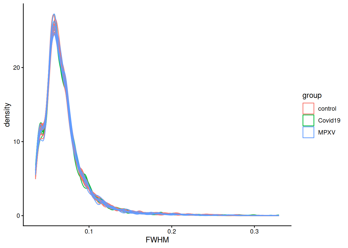
2.7 Save data
TipKey Points
- DIA-NN outputs a
.parquetformat report file containing precursor- and protein-level quantification data for each sample - The
readQFeaturesFromDIANNfunction imports DIA-NN output into aQFeaturesobject, creating oneSummarizedExperimentper sample run - Sample metadata is stored in the
colDataof theQFeaturesobject and can be used to annotate samples with experimental group information - The
rowDataof each per-sampleSummarizedExperimentcontains quality metrics from DIA-NN (e.g. FWHM, Q-values) that can be used to explore data quality and guide downstream filtering decisions