Know how to use filterFeatures to filter DIA-NN precursor data by Q-value thresholds
Know how to use joinAssays to combine per-sample SummarizedExperiment objects into a single combined set
Know how to identify and remove contaminant proteins
Be able to explore and visualise missing values in DIA proteomics data
Understand how to filter sparse precursors based on a missing value threshold
Now that we have our precursor-level data stored in a QFeatures object, the next step is to carry out data cleaning — filtering to retain only high-confidence identifications and removing precursors with excessive missing values across samples.
3.1 Filtering by Q-value
Discussion
Before reading on, consider the following:
Why do we need to filter the DIA-NN output at all? What would happen if we kept all identifications?
What do the Q-value columns represent, and what is the difference between run-level and library-level Q-values?
What threshold would you choose?
What impact could this filtering have on the downstream analysis and results?
DIA-NN assigns a Q-value to each precursor and protein group identification, representing the local false discovery rate (FDR) at that score threshold — i.e., the expected proportion of identifications at that level that are incorrect. Filtering by Q-value ensures we retain only high-confidence identifications before proceeding to downstream analysis.
DIA-NN outputs several Q-value columns:
Q.Value — run-level precursor Q-value (FDR within a single run)
PG.Q.Value — run-level protein group Q-value
Lib.Q.Value — library-level precursor Q-value (based on the spectral library used in matching)
Lib.PG.Q.Value — library-level protein group Q-value
Since our data was processed with match-between-runs (MBR) enabled, we additionally filter on the library-level Q-values (Lib.Q.Value and Lib.PG.Q.Value). When MBR is used, DIA-NN rescores identifications across runs using an empirical library built in a first pass; the library-level Q-values reflect the confidence of those cross-run matches and are therefore the most stringent and appropriate filter for MBR data. We apply a standard 1% FDR threshold (Q-value ≤ 0.01) to all four columns.
To remove features based on variables within our rowData we make use of the filterFeatures function. This function takes a QFeatures object as its input and filters it against a condition based on the rowData (indicated by the ~ operator). If the condition evaluates to TRUE for a feature, that feature will be kept; features returning FALSE are removed.
The filterFeatures function provides the option to apply a filter either (i) to the whole QFeatures object and all of its SummarizedExperiments, or (ii) to specific SummarizedExperiments within the QFeatures object, by passing the name or index of the desired set to the i argument.
Since we want to apply the Q-value filter across all per-sample SummarizedExperiments simultaneously, we do not pass an i argument — this causes filterFeatures to apply the filter to every set in the QFeatures object.
dia_qf
An instance of class QFeatures (type: bulk) with 31 sets:

 [1] COVID_E1: SummarizedExperiment with 3834 rows and 1 columns
 [2] COVID_E10: SummarizedExperiment with 3914 rows and 1 columns
 [3] COVID_E2: SummarizedExperiment with 4016 rows and 1 columns
 ...
 [29] MPX_D4: SummarizedExperiment with 3950 rows and 1 columns
 [30] MPX_D5: SummarizedExperiment with 4043 rows and 1 columns
 [31] MPX_D6: SummarizedExperiment with 3861 rows and 1 columns
dia_qf <- dia_qf %>%filterFeatures(~ Q.Value <=0.01) %>%# Run-level precursor Q-valuefilterFeatures(~ PG.Q.Value <=0.01) %>%# Run-level protein group Q-valuefilterFeatures(~ Lib.Q.Value <=0.01) %>%# Library-level precursor Q-valuefilterFeatures(~ Lib.PG.Q.Value <=0.01) # Library-level protein group Q-value
'Q.Value' found in 31 out of 31 assay(s).
'PG.Q.Value' found in 31 out of 31 assay(s).
'Lib.Q.Value' found in 31 out of 31 assay(s).
'Lib.PG.Q.Value' found in 31 out of 31 assay(s).
dia_qf
An instance of class QFeatures (type: bulk) with 31 sets:

 [1] COVID_E1: SummarizedExperiment with 3751 rows and 1 columns
 [2] COVID_E10: SummarizedExperiment with 3851 rows and 1 columns
 [3] COVID_E2: SummarizedExperiment with 3910 rows and 1 columns
 ...
 [29] MPX_D4: SummarizedExperiment with 3882 rows and 1 columns
 [30] MPX_D5: SummarizedExperiment with 3971 rows and 1 columns
 [31] MPX_D6: SummarizedExperiment with 3788 rows and 1 columns
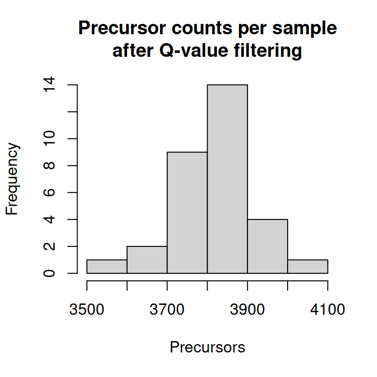
We can see how many precursors remain per sample after filtering by inspecting the number of rows in each per-sample set.
hist(nrows(dia_qf),xlab ="Precursors",main ="Precursor counts per sample\nafter Q-value filtering")
3.2 Joining per-sample sets into a single precursor set
After filtering, our QFeatures object contains one SummarizedExperiment per sample run. To work with the data combined across all samples, we use the joinAssays function. This merges all per-sample sets into a single combined set called "precursors", aligning features (precursors) by their Precursor.Id. Where a precursor was not detected in a particular sample, the corresponding entry will be NA.
Note that joinAssays only retains rowData columns that are shared across all sets and have consistent values — run-specific metrics such as Q.Value, PEP, and Run are therefore dropped from the combined set. This is expected: these per-run quality metrics were used for filtering in the previous step and are no longer needed. We can confirm which columns are dropped by comparing the rowData names before and after joining.
# rowData columns in the per-sample setssample_level_rdata_names <-rowDataNames(dia_qf)[[1]]# rowData columns in the combined setjoined_rdata_names <-rowDataNames(dia_qf)[["precursors"]]# Columns present in sample-level sets but dropped from the combined setsetdiff(sample_level_rdata_names, joined_rdata_names)
Now that the per-sample data has been joined into the "precursors" set, we no longer need to keep the individual per-sample SummarizedExperiment objects. To reduce the size of our QFeatures object, we identify the sets for individual samples and remove them. This isn’t strictly necessary for this dataset, but it may be if you have a very large experiment. It also helps to keep the object tidy and focused on the combined set for downstream analysis.
The sampleMap is an internal table in a QFeatures object that records which samples are present in each assay. We can inspect it before removing the per-sample sets — at this point it contains one row per sample per assay, so with 31 samples, it has 62 rows - one row each for the original per-sample assay and for the "precursors" assay.
After calling removeAssay, the 31 per-sample assays are dropped and their corresponding sampleMap entries are removed, leaving only the rows for "precursors". You will see a message indicating that sampleMap rows have been harmonised — this is expected behaviour.
sets_to_rm <-which(names(dia_qf) !="precursors")dia_qf <-removeAssay(dia_qf, i = sets_to_rm)
Warning: 'experiments' dropped; see 'drops()'
harmonizing input:
  removing 31 sampleMap rows not in names(experiments)
In any proteomics experiment, some identified peptides will derive from contaminant proteins rather than the sample of biological interest. Common contaminants include proteins introduced during sample preparation — for example, human keratins from skin or hair, bovine serum albumin from cell culture media, and trypsin used for proteolytic digestion. These proteins are not informative for the biological question and should be removed before downstream analysis.
It is standard practice to include a curated contaminants database alongside the primary sequence database during the database search. For this data, we used a modified version of the contaminants fasta from Hao Group’s Protein Contaminant Libraries for DDA and DIA ProteomicsFrankenfield et al. (2022), where we removed the contaminants from Fetal Bovine Serum, which are not relevant here. The entries in this contaminant database are named with a Cont_ prefix, which is carried through into the Protein.Ids column of the DIA-NN output, making them straightforward to identify computationally.
We can inspect the rowData to check the contaminants can be identified as expected.
It’s important to note that because DIA-NN uses a normalisation based on total sample intensity under the assumption that the same amount of peptides were injected in each sample, precursors mapping to contaminants included in the FASTA database are excluded from quantification.
# Extract the rowDatard <-rowData(dia_qf[['precursors']]) %>%data.frame()table(grepl('Cont_', rd$Protein.Ids))
FALSE  TRUE
 4417   275
3.5 Filtering contaminants
We now remove precursors with a contaminant match from our data.
As with all data analyses, it is sensible to keep a copy of the data before applying filters, in case we need to refer back to the unfiltered data later. We therefore extract a copy of the set using addAssay, giving it a new name that reflects the processing step we are about to apply. We will only apply filters to this new copy, leaving the original set untouched.
NoteAssay links
QFeatures maintains hierarchical links between quantitative levels, allowing easy access to all data levels for individual features of interest. This is fundamental to the QFeatures infrastructure and will be exemplified throughout this course. When using addAssay to add a copy of an existing set, the newly created SummarizedExperiment does not automatically have a link to the set it was copied from. Where a link is required, it can be added explicitly using addAssayLink.
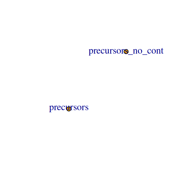
We create a copy of the "precursors" set called "precursors_no_cont". After filtering, this set will contain only precursors do not originate from contaminants. We use plot to visualise the assay structure before and after adding the link.
dia_qf <-addAssay(dia_qf, dia_qf[["precursors"]], name ="precursors_no_cont")plot(dia_qf)
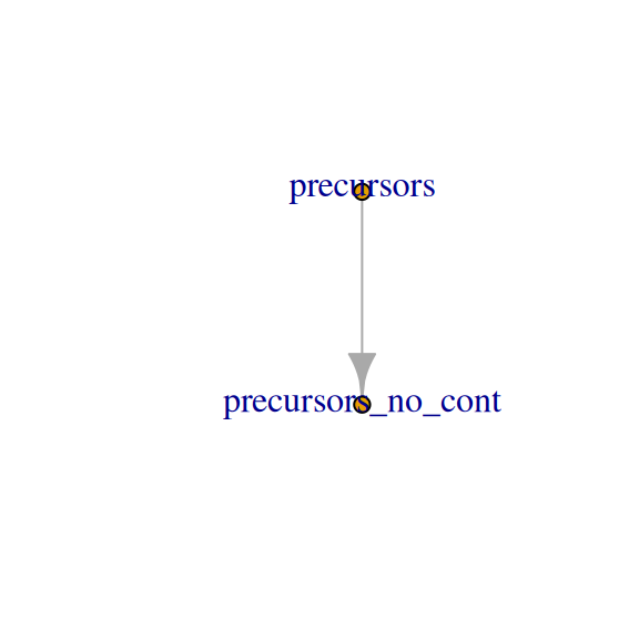
dia_qf <-addAssayLink(dia_qf, from ="precursors", to ="precursors_no_cont")plot(dia_qf)
We then use filterFeatures to retain only precursors whose Protein.Ids field contains no Cont_ entry. We specifying the i argument to apply the filter only to the "precursors_no_cont" set. This retains the original "precursors" assay with all precursors for reference, while the new set contains only those precursors that pass the missing value threshold.
An instance of class QFeatures (type: bulk) with 2 sets:

 [1] precursors: SummarizedExperiment with 4692 rows and 31 columns
 [2] precursors_no_cont: SummarizedExperiment with 4417 rows and 31 columns
3.6 Exploring missing values
DIA proteomics data can exhibit substantial missing values because proteins must be detected independently in each sample run. Before filtering, it is important to understand the extent and distribution of missing values in the data.
We use the nNA function to calculate the proportion of missing values per precursor (row) and per sample (column).
precursors_missing <-nNA(dia_qf, i ="precursors_no_cont")print(precursors_missing)
Using the precursors_missing object, create plots to explore the distribution of missing values in the data.
Plot a histogram for the proportion of missing values across precursors.
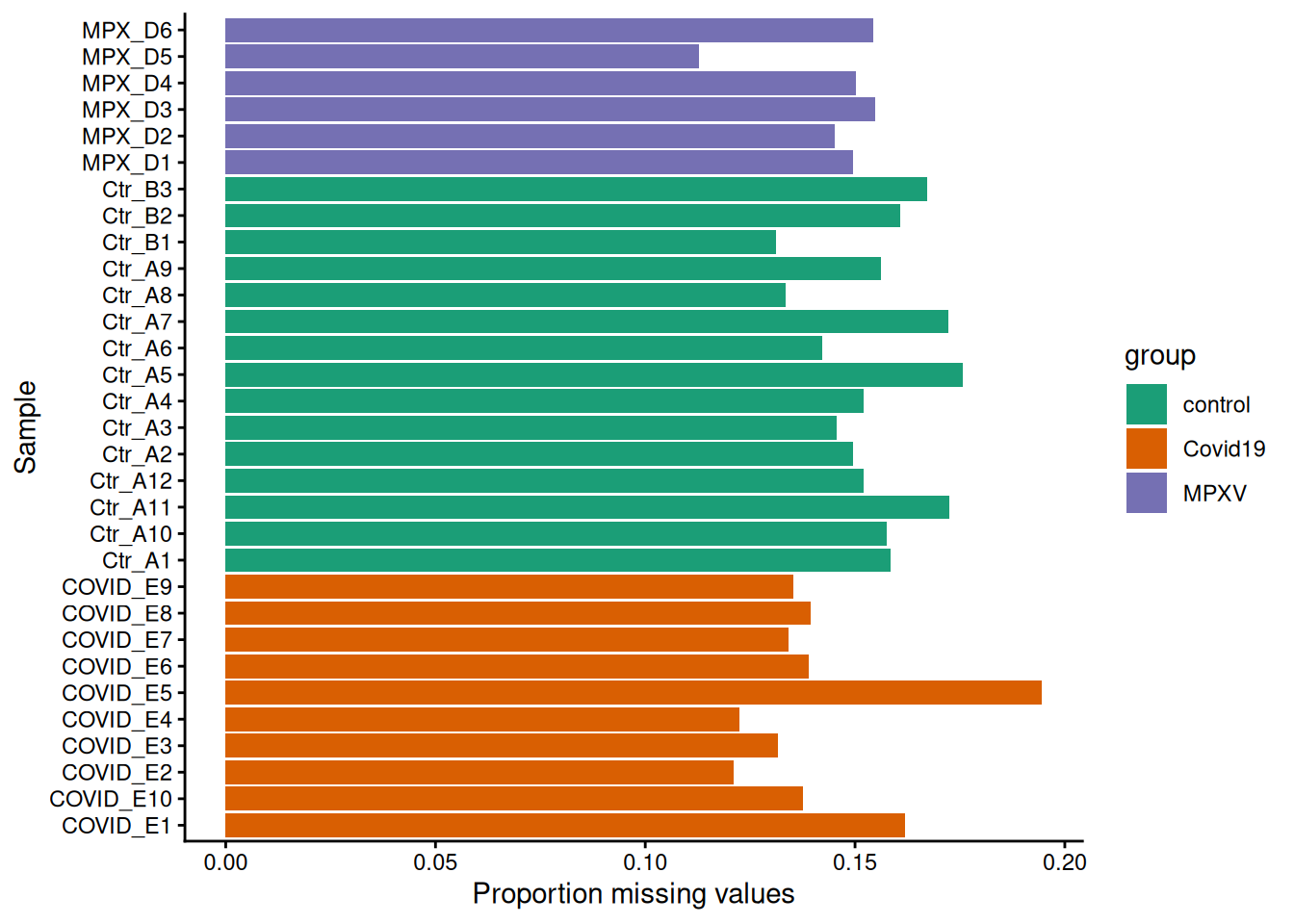
Plot the proportion of missing values per sample, coloured by group.
Based on your plots:
Do most precursors have missing values?
Are there any precursors or samples with an unusually high proportion of missing values?
Does the proportion of missing values differ between groups?
Hint
The precursors_missing object contains two data frames: nNArows (one row per precursor) and nNAcols (one row per sample), each with a pNA column giving the proportion of missing values.
AnswerAnswer
Task 1
hist( precursors_missing$nNArows$pNA,xlab ="Proportion missing values",main ="Missing values per precursor")
Task 2
precursors_missing$nNAcols %>%as_tibble() %>%merge(data.frame(colData(dia_qf)), by.x ="name", by.y ="runCol") %>%ggplot(aes(x = name, y = pNA, group = group, fill = group)) +geom_bar(stat ="identity") +labs(x ="Sample", y ="Proportion missing values") +coord_flip() +scale_fill_brewer(palette ="Dark2") +theme_classic()
Precursors that are missing across the majority of samples provide little useful quantitative information and may introduce noise into downstream analyses. We filter out precursors with excessive missing values using the filterNA function, where the pNA argument specifies the maximum proportion of missing values allowed per precursor.
The choice of threshold involves a trade-off: stricter thresholds (lower pNA) remove more precursors and produce a cleaner but smaller dataset; more permissive thresholds retain more precursors but include those with very sparse quantification, which are more likely to be inaccurately quantified. Here we use pNA = 0.75, meaning a precursor must be observed in at least 25% of samples — with 31 samples, this corresponds to a minimum of approximately 8 observations. Further filtering will be applied at the protein level in the statistical analysis, where we will require proteins to be quantified in at least 3 replicates per group before testing.
3.7 Filtering sparse precursors
We create a copy called "precursors_filtered_missing" — after filtering, this set will contain only precursors that meet the missing value threshold.
Now we perform the missing value filtering on the new assay, again specifying the i argument to apply the filter to only the desired set.
dia_qf <- dia_qf %>%filterNA(pNA =0.75, i ="precursors_filtered_missing")
3.8 Save data
TipKey Points
DIA-NN Q-value columns (Q.Value, PG.Q.Value, Lib.Q.Value, Lib.PG.Q.Value) represent the local FDR for each identification; filtering at ≤ 0.01 retains only identifications at 1% FDR
When match-between-runs is enabled, library-level Q-values (Lib.Q.Value, Lib.PG.Q.Value) are the most appropriate filter as they reflect the confidence of cross-run matches
filterFeatures applies row-level filters based on rowData variables, and can be applied to the whole QFeatures object or to specific sets
Contaminant proteins (e.g., keratins, trypsin, BSA) should be removed before downstream analysis; including a curated contaminant database in the search and filtering on a Cont_ prefix in Protein.Ids is a straightforward way to do this
joinAssays combines per-sample SummarizedExperiment objects into a single combined set, with missing values (NA) where a precursor was not detected in a given sample
nNA provides a convenient summary of missing values per feature (row) and per sample (column)
DIA data typically has a relatively high proportion of missing values, as proteins must be detected independently in each sample
filterNA removes precursors that are missing above a specified proportion of samples, with the threshold chosen based on the experimental context
References
Frankenfield, Ashley M., Jiawei Ni, Mustafa Ahmed, and Ling Hao. 2022. “Protein Contaminants Matter: Building Universal Protein Contaminant Libraries for DDA and DIA Proteomics.”Journal of Proteome Research 21 (9): 2104–13. https://doi.org/10.1021/acs.jproteome.2c00145.