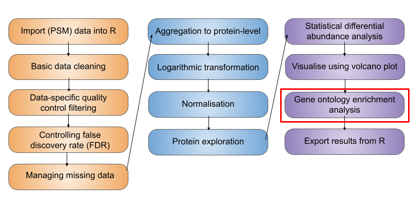
7 Biological interpretation
TipLearning Objectives
- Be aware of different analyses that can be done to gain a biological understanding of expression proteomics results
- Understand the concept of Gene Ontology (GO) enrichment analyses
- Complete GO enrichment analyses using the
enrichGOfunction from theclusterProfilerpackage
7.1 Adding metadata to our results using dplyr
Before we can look any further into the biological meaning of any protein abundance changes we need to extract these proteins from our overall results. It is also useful to re-add information about the master protein descriptions since this is lost in the output of limma analysis.
It is important to note that the results table we have generated from limma is not in the same order as the input data. Therefore, to add information from our original data e.g., from the rowData such as the Master.Protein.Descriptions we must match the protein names between them.
To do this, let’s extract information the Master.Protein.Descriptions from the original data we have created called all_proteins.
Recall that all_proteins is a SummarizedExperiment object,
all_proteinsclass: SummarizedExperiment
dim: 3823 6
metadata(0):
assays(2): assay aggcounts
rownames(3823): A0A0B4J2D5 A0A2R8Y4L2 ... Q9Y6X9 Q9Y6Y8
rowData names(21): Checked Tags ... Protein.FDR.Confidence .n
colnames(6): M_1 M_2 ... G1_2 G1_3
colData names(4): sample rep condition tagWe wish to extract information from the rowData regarding the Master.Protein.Descriptions,
## Add master protein descriptions back
protein_info <- all_proteins %>%
  rowData() %>%
  as_tibble() %>%
  select(Protein = Master.Protein.Accessions,
         Protein_description = Master.Protein.Descriptions)

protein_info %>% head()
# A tibble: 6 × 2
Protein Protein_description
<chr> <chr>
1 A0A0B4J2D5 Putative glutamine amidotransferase-like class 1 domain-containing…
2 A0A2R8Y4L2 Heterogeneous nuclear ribonucleoprotein A1-like 3 OS=Homo sapiens …
3 A0AVT1 Ubiquitin-like modifier-activating enzyme 6 OS=Homo sapiens OX=960…
4 A0MZ66 Shootin-1 OS=Homo sapiens OX=9606 GN=SHTN1 PE=1 SV=4
5 A1L0T0 2-hydroxyacyl-CoA lyase 2 OS=Homo sapiens OX=9606 GN=ILVBL PE=1 SV…
6 A1X283 SH3 and PX domain-containing protein 2B OS=Homo sapiens OX=9606 GN…Note, we also extract the Master.Protein.Accessions column so we can use this to match to the protein column in our limma results.
Now we can use the left_join function from dplyr to match the protein descriptions to the protein IDs,
limma_results <- limma_results %>%
  left_join(protein_info, by = "Protein", suffix = c(".left", ".right"))

# Verify
limma_results %>%
  head()
Protein logFC AveExpr t P.Value adj.P.Val B
1 Q9NQW6 -2.077921 2.641270 -40.40812 1.139582e-15 4.356623e-12 25.79468
2 Q9BW19 -2.343592 1.430210 -36.79774 4.073530e-15 7.786553e-12 24.71272
3 P49454 -1.991326 2.598481 -34.88623 8.411188e-15 9.266757e-12 24.07905
4 Q9ULW0 -2.152503 2.476087 -34.52309 9.695796e-15 9.266757e-12 23.95341
5 Q562F6 -3.205603 -1.304111 -32.91865 1.849860e-14 1.414403e-11 23.37677
6 O14965 -2.098029 0.797902 -31.22180 3.791132e-14 2.415583e-11 22.72604
direction significance
1 down sig
2 down sig
3 down sig
4 down sig
5 down sig
6 down sig
Protein_description
1 Anillin OS=Homo sapiens OX=9606 GN=ANLN PE=1 SV=2
2 Kinesin-like protein KIFC1 OS=Homo sapiens OX=9606 GN=KIFC1 PE=1 SV=2
3 Centromere protein F OS=Homo sapiens OX=9606 GN=CENPF PE=1 SV=3
4 Targeting protein for Xklp2 OS=Homo sapiens OX=9606 GN=TPX2 PE=1 SV=2
5 Shugoshin 2 OS=Homo sapiens OX=9606 GN=SGO2 PE=1 SV=2
6 Aurora kinase A OS=Homo sapiens OX=9606 GN=AURKA PE=1 SV=3
NoteManipulating data with
dplyr and tidyverse
There is lots of information online about getting started with dplyr and using the tidyverse. We really like this lesson from the Data Carpentry if you are new to the tidyverse.
7.2 Subset differentially abundant proteins
Let’s subset our results and only keep proteins which have been flagged as exhibiting significant abundance changes,
sig_changing <- limma_results %>%
  as_tibble() %>%
  filter(significance == "sig")

sig_up <- sig_changing %>%
  filter(direction == "up")

sig_down <- sig_changing %>%
  filter(direction == "down")
7.3 Biological interpretation of differentially abundant proteins
Our statistical analyses provided us with a list of proteins that are present with significantly different abundances between M-phase and G1-phase of the cell cycle. We can get an initial idea about what these proteins are and do by looking at the protein descriptions.
## Look at descriptions of proteins upregulated in M relative to G1
sig_up %>%
  pull(Protein_description) %>%
  head()
[1] "Golgi reassembly-stacking protein 2 OS=Homo sapiens OX=9606 GN=GORASP2 PE=1 SV=3"
[2] "Selenoprotein S OS=Homo sapiens OX=9606 GN=SELENOS PE=1 SV=3"
[3] "Anamorsin OS=Homo sapiens OX=9606 GN=CIAPIN1 PE=1 SV=2"
[4] "Krueppel-like factor 16 OS=Homo sapiens OX=9606 GN=KLF16 PE=1 SV=1"
[5] "Histone H1.10 OS=Homo sapiens OX=9606 GN=H1-10 PE=1 SV=1"
[6] "Importin subunit alpha-4 OS=Homo sapiens OX=9606 GN=KPNA3 PE=1 SV=2" Whilst we may recognise some of the changing proteins, this might be the first time that we are coming across others. Moreover, some protein descriptions contain useful information, but this is very limited. We still want to find out more about the biological role of the statistically significant proteins so that we can infer the potential effects of their abundance changes.
There are many functional analyses that could be done on the proteins with differential abundance:
- Investigate the biological pathways that the proteins function within (KEGG etc.)
- Identify potential interacting partners (IntAct, STRING)
- Determine the subcellular localisation in which the changing proteins are found
- Understand the co-regulation of their mRNAs (Expression Atlas)
- Compare our changing proteins to those previously identified in other proteomic studies of the cell cycle
7.3.1 Gene Ontology (GO) enrichment analysis
One of the common methods used to probe the biological relevance of proteins with significant changes in abundance between conditions is to carry out Gene Ontology (GO) enrichment, or over-representation, analysis.
The Gene Ontology consortium have defined a set of hierarchical descriptions to be assigned to genes and their resulting proteins. These descriptions are split into three categories: cellular components (CC), biological processes (BP) and molecular function (MF). The idea is to provide information about a protein’s subcellular localisation, functionality and which processes it contributes to within the cell. Hence, the overarching aim of GO enrichment analysis is to answer the question:
“Given a list of proteins found to be differentially abundant in my phenotype of interest, what are the cellular components, molecular functions and biological processes involved in this phenotype?”.
Unfortunately, just looking at the GO terms associated with our differentially abundant proteins is insufficient to draw any solid conclusions. For example, if we find that 120 of the 453 proteins significantly downregulated in M phase are annotated with the GO term “kinase activity”, it may seem intuitive to conclude that reducing kinase activity is important for the M-phase phenotype. However, if 90% of all proteins in the cell were kinases (an extreme example), then we might expect to discover a high representation of the “kinase activity” GO term in any protein list we end up with.
This leads us to the concept of an over-representation analysis. We wish to ask whether any GO terms are over-represented (i.e., present at a higher frequency than expected by chance) in our lists of differentially abundant proteins. In other words, we need to know how many proteins with a GO term could have shown differential abundance in our experiment vs. how many proteins with this GO term did show differential abundance in our experiment.
We are going to use a function in R called enrichGO from the the clusterProfiler Yu et al. (2012) Bioconductor R package to perform GO enrichment analysis. The package vignette can be found here. and full tutorials for using the package here
NoteAnnotation packages in Bioconductor
The enrichGO function uses the org.Hs.eg.db Bioconductor package that has genome wide annotation for human. It also uses the GO.db package which is a set of annotation maps describing the entire Gene Ontology assembled using data from GO.
Unfortunately, because GO annotations are by design at the gene level, performing analyses with proteomics data can be more tricky.
In the next code chunk we call the enrichGO function.
ego_down <- enrichGO(gene = sig_down$Protein,               # list of down proteins
                     universe = limma_results$Protein,      # all proteins
                     OrgDb = org.Hs.eg.db,                  # database to query
                     keyType = "UNIPROT",                   # protein ID encoding
                     qvalueCutoff = 0.05,
                     ont = "BP",                            # can be CC, MF, BP, or ALL
                     readable = TRUE)
Let’s take a look at the output.
head(ego_down@result) ID Description GeneRatio
GO:0030198 GO:0030198 extracellular matrix organization 24/443
GO:0043062 GO:0043062 extracellular structure organization 24/443
GO:0045229 GO:0045229 external encapsulating structure organization 24/443
GO:0055085 GO:0055085 transmembrane transport 61/443
GO:0045333 GO:0045333 cellular respiration 35/443
GO:0030199 GO:0030199 collagen fibril organization 13/443
BgRatio RichFactor FoldEnrichment zScore pvalue
GO:0030198 52/3673 0.4615385 3.826706 7.601862 8.298786e-10
GO:0043062 52/3673 0.4615385 3.826706 7.601862 8.298786e-10
GO:0045229 52/3673 0.4615385 3.826706 7.601862 8.298786e-10
GO:0055085 244/3673 0.2500000 2.072799 6.422166 5.339347e-09
GO:0045333 107/3673 0.3271028 2.712074 6.655422 9.470160e-09
GO:0030199 19/3673 0.6842105 5.672924 7.561939 1.326766e-08
p.adjust qvalue
GO:0030198 7.753832e-07 6.563320e-07
GO:0043062 7.753832e-07 6.563320e-07
GO:0045229 7.753832e-07 6.563320e-07
GO:0055085 3.741547e-06 3.167076e-06
GO:0045333 5.308972e-06 4.493840e-06
GO:0030199 6.198208e-06 5.246545e-06
geneID
GO:0030198 CCN1/QSOX1/COL12A1/ITGB1/SERPINH1/APP/LAMC1/PLOD2/COL23A1/P4HA1/FLOT1/LOXL2/COL4A2/FKBP10/PLOD1/MMP2/CRTAP/PRDX4/COLGALT1/PLOD3/TGFB2/ERO1A/COL1A1/DAG1
GO:0043062 CCN1/QSOX1/COL12A1/ITGB1/SERPINH1/APP/LAMC1/PLOD2/COL23A1/P4HA1/FLOT1/LOXL2/COL4A2/FKBP10/PLOD1/MMP2/CRTAP/PRDX4/COLGALT1/PLOD3/TGFB2/ERO1A/COL1A1/DAG1
GO:0045229 CCN1/QSOX1/COL12A1/ITGB1/SERPINH1/APP/LAMC1/PLOD2/COL23A1/P4HA1/FLOT1/LOXL2/COL4A2/FKBP10/PLOD1/MMP2/CRTAP/PRDX4/COLGALT1/PLOD3/TGFB2/ERO1A/COL1A1/DAG1
GO:0055085 THBS1/ITGB1/HSPA5/RACGAP1/TOMM70/MAGT1/ATP5F1A/SLC3A2/ATP1B1/SLC39A14/SLC2A1/HSPD1/SLC29A1/TIMM50/HSPA9/ASPH/TIMM21/ITGAV/NDUFS2/AIFM1/USP9X/TMEM165/SLC12A2/NNT/FLNA/PEX14/AFG3L2/UQCRC1/SLC25A3/NDUFS7/RALBP1/YES1/ATP5F1B/ERO1A/ARPP19/FMR1/ABCB7/GHITM/MT-CO2/ATP2A2/GRPEL1/ATP2B1/SLC25A24/TIMM44/ATP1A1/ATP6AP2/LETM1/SLC7A1/GOPC/ATP5PB/RPS6KB1/NDUFB3/UQCRFS1/TOMM40/ACTN4/COX4I1/SLC30A1/PMPCB/NDUFB8/STXBP3/SLC1A5
GO:0045333 PLEC/ATP5F1A/CS/SOD2/SDHA/ACO2/SHMT2/NDUFS2/NNT/NDUFB11/ETFA/MDH2/SDHB/SUCLA2/UQCRC1/UQCRC2/CDK1/NDUFS7/SUCLG2/ATP5F1B/GHITM/MT-CO2/DLST/DLD/OXA1L/IDH3A/ATP5PB/STOML2/NDUFB3/CAT/HCCS/UQCRFS1/PDHB/COX4I1/NDUFB8
GO:0030199 COL12A1/SERPINH1/PLOD2/P4HA1/LOXL2/FKBP10/PLOD1/CRTAP/COLGALT1/PLOD3/TGFB2/ERO1A/COL1A1
Count
GO:0030198 24
GO:0043062 24
GO:0045229 24
GO:0055085 61
GO:0045333 35
GO:0030199 13The output of the enrichGO function is an object of class enrichResult that contains the ID and Description of all enriched GO terms. There is also information about which geneIDs from our significantly downregulated proteins are annotated with each of the enriched GO terms. Let’s take a look at the descriptions.
ego_down$Description %>%
  head(10)
[1] "extracellular matrix organization"
[2] "extracellular structure organization"
[3] "external encapsulating structure organization"
[4] "transmembrane transport"
[5] "cellular respiration"
[6] "collagen fibril organization"
[7] "cell adhesion"
[8] "mitochondrial transmembrane transport"
[9] "cell division"
[10] "aerobic respiration" There is a long list because of the hierarchical nature of GO terms. The results of GO enrichment analysis can be visualised in many different ways. For a full overview of GO enrichment visualisation tools see Visualization of functional enrichment result.
Here, we’ll use a ‘dotplot’ first
p <- dotplot(ego_down,
        x = "Count",
        showCategory = 20,
        font.size = 10,
        label_format = 100,
        color = "p.adjust")

print(p)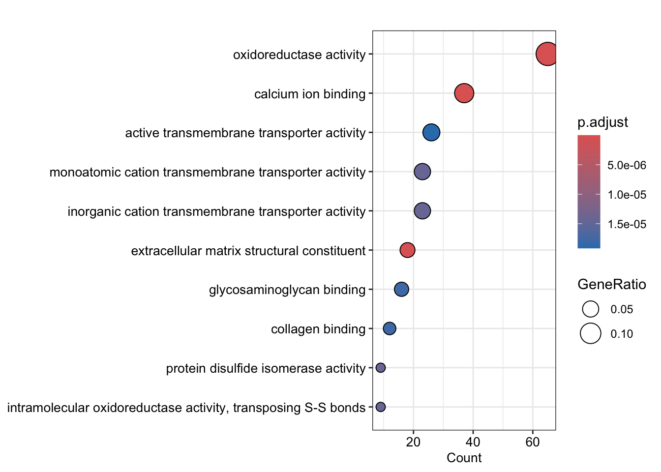
The dotplot gives a good overview of the over-representation results for the top GO terms, but it’s not clear how much overlap there is between the proteins annotated with each term. For this, we can use an ‘upset’ plot.
upsetplot(ego_down, n=10)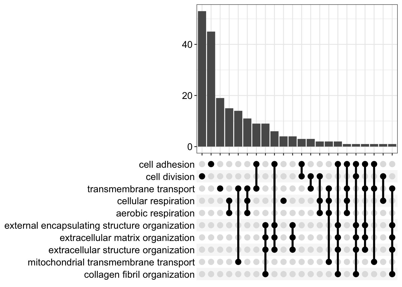
It’s usually informative to explore the proteins with the over-represented GO terms further. For this, we need to know which proteins have a particular GO term. This is where is gets a little more tricky, since we need to map between Uniprot IDs and Entrez gene IDs for this.
We start by using the toTable method to turn the UNIPROT map into a data.frame.
## Obtain a gene to protein mapping for the proteins in our QFeatures
## org.Hs.egUNIPROT is part of org.Hs.eg.db
g2p_map_df <- toTable(org.Hs.egUNIPROT) %>%
  filter(uniprot_id %in% rownames(cc_qf[['log_norm_proteins']]))

## Obtain the GO terms for each gene
go_submap <- org.Hs.egGO[g2p_map_df$gene_id]

## Merge the gene to protein map and GO terms for
## genes to get GO terms for proteins
p2go <- toTable(go_submap) %>%
  left_join(g2p_map_df, by='gene_id')
Warning in left_join(., g2p_map_df, by = "gene_id"): Detected an unexpected many-to-many relationship between `x` and `y`.
ℹ Row 33120 of `x` matches multiple rows in `y`.
ℹ Row 186 of `y` matches multiple rows in `x`.
ℹ If a many-to-many relationship is expected, set `relationship =
"many-to-many"` to silence this warning.Now we can visualise the proteins with a particular GO term. Here, we will use a heatmap to see the patterns in protein abundance differences between the conditions for a given GO term.
ExerciseExercise 1 - Challenge: Plot a heatmap for the significant cell division proteins
Level:
Make a heatmap with the protein abundances in all samples for those proteins with ‘cell division’ GO annotation. You can use the ego_down@result data.frame to get the GO term for ‘cell division’, or, failing that, your favourite search engine. For the heatmap plotting, you can refer back to the end of the previous session where we used pheatmap.
- How does the protein abundance in the desyncronised cells compare to the M/G1 phases? How does this inform your interpretation?
AnswerAnswer
## Get the GO ID for 'cell division'
cell_division_go <- ego_down@result %>%
  filter(Description=='cell division') %>%
  rownames()

## Get the Uniprot IDs for cell division annotated proteins
cell_division_uniprot_ids <- p2go %>%
  filter(go_id==cell_division_go) %>%
  pull(uniprot_id) %>%
  unique()

## Extract quant data
quant_data <- cc_qf[["log_norm_proteins"]] %>% assay()

## Plot heatmap
pheatmap(mat = quant_data,
         scale = "row",
         show_rownames = FALSE)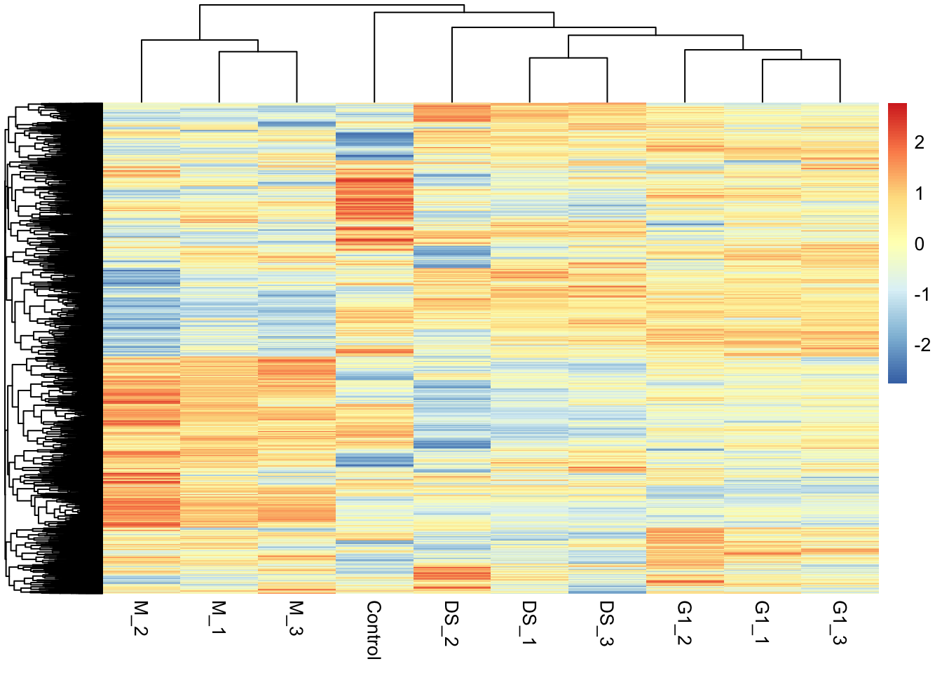
## Extract quant data for the significant proteins
quant_data_cd <- quant_data[intersect(sig_changing$Protein, cell_division_uniprot_ids), ]

## Plot heatmap
pheatmap(mat = quant_data_cd,
         scale = "row",
         show_rownames = TRUE)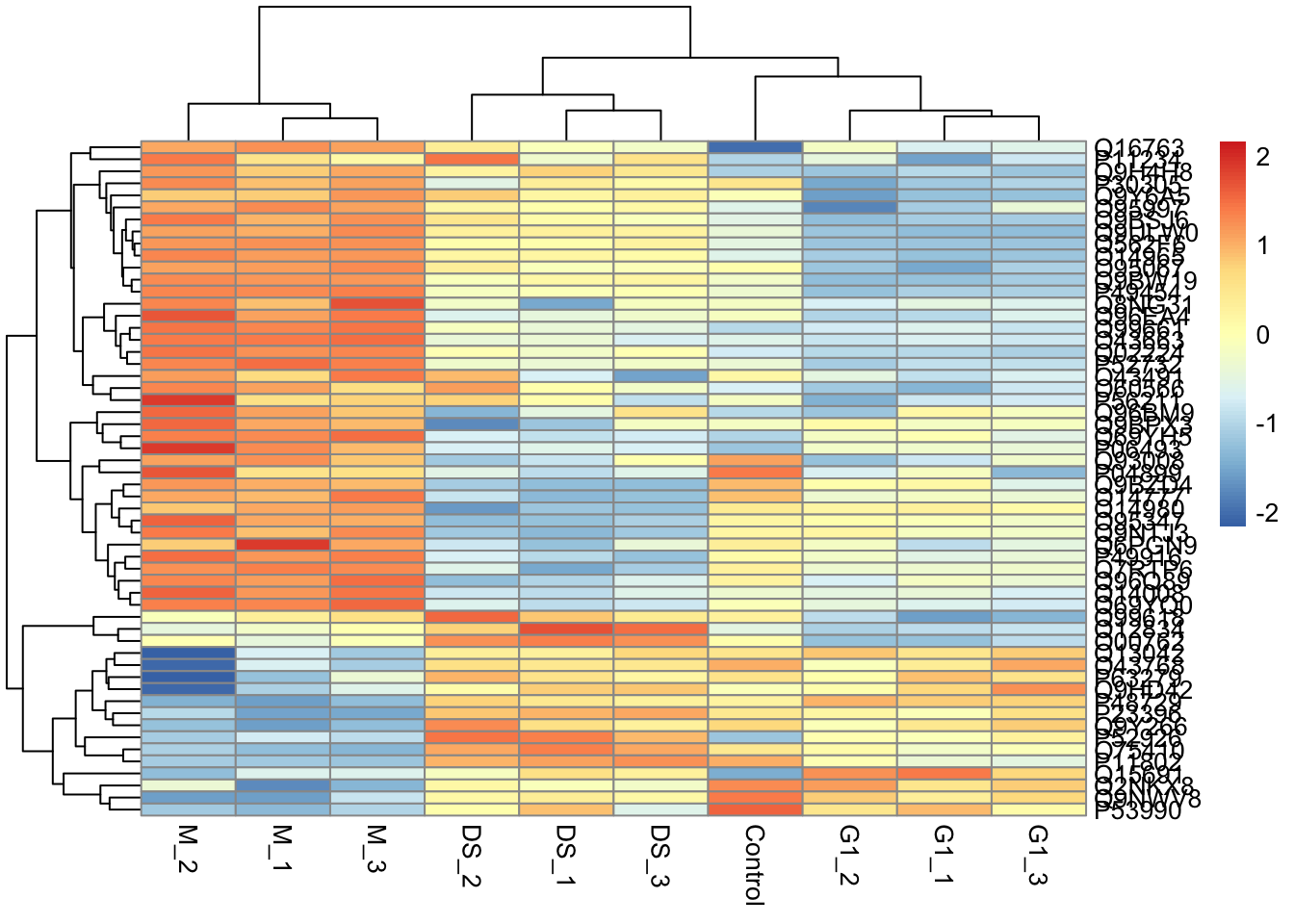
TipKey Points
- Gene ontology (GO) terms described the molecular function (MF), biological processes (BP) and cellular component (CC) of genes (and their protein products).
- GO terms are hierarchical and generic. They do not relate to specific biological systems e.g., cell type or condition.
- GO enrichment analysis aims to identify GO terms that are present in a list of proteins of interest (foreground) at a higher frequency than expected by chance based on their frequency in a background list of proteins (universe). The universe should be a list of all proteins included identified and quantified in your experiment.
- The
enrichGOfunction from theclusterProfilerpackage provides a convenient way to carry out reproducible GO enrichment analysis in R. - There are many ways to visualise the results from functional enrichment analyses. With GO terms in particular, it’s important to consider the relationships between the gene sets we are testing for over-representation.
References
Yu, Guangchuang, Li-Gen Wang, Yanyan Han, and Qing-Yu He. 2012. “clusterProfiler: An r Package for Comparing Biological Themes Among Gene Clusters.” OMICS: A Journal of Integrative Biology 16 (5): 284–87. https://doi.org/10.1089/omi.2011.0118.