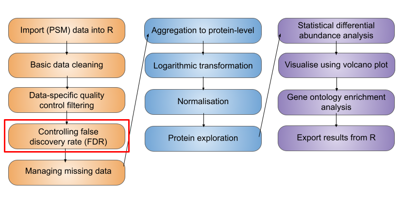
3 Data cleaning
TipLearning Objectives
- Be aware of key data cleaning steps which should or could be completed during the processing of expression proteomics data
- Make use of the
filterFeaturesfunction to conditionally remove data from (i) an entireQFeaturesobject or (ii) specifiedSummarizedExperimentof aQFeaturesobject - Understand the difference between non-specific and data-dependent filtering
- Be able to explore the feature data stored in the
rowDataand get a feel for how to make your own data-dependent decisions regarding data cleaning - Understand the importance of dealing with missing values in expression proteomics datasets and be aware of different approaches to doing so
Now that we have our PSM level quantitative data stored in a QFeatures object, the next step is to carry out some data cleaning. However, as with all data analyses, it is sensible to keep a copy of our raw data in case we need to refer back to it later.
3.1 Creating a copy of the raw data
To create a copy of the psms_raw data we can first extract the SummarizedExperiment and then add it back to our QFeatures object using the addAssay function. When we do this, we give the second SummarizedExperiment (our copy) a new name. Here we will call it psms_filtered as by the end of our data cleaning and filtering, this copy will have had the unwanted data removed.
## Extract a copy of the raw PSM-level data
raw_data_copy <- cc_qf[["psms_raw"]]

## Re-add the assay to our QFeatures object with a new name
cc_qf <- addAssay(x = cc_qf,
                  y = raw_data_copy,
                  name = "psms_filtered")

## Verify
cc_qf
An instance of class QFeatures (type: bulk) with 2 sets:
[1] psms_raw: SummarizedExperiment with 45803 rows and 10 columns
[2] psms_filtered: SummarizedExperiment with 45803 rows and 10 columns We now see that a second SummarizedExperiment has been added to the QFeatures object. When we use addAssay to add to a QFeatures object, the newly created SummarizedExperiment does not automatically have links to the pre-existing SummarizedExperiments.
NoteAssay links
QFeatures maintains the hierarchical links between quantitative levels whilst allowing easy access to all data levels for individual features (PSMs, peptides and proteins) of interest. This is fundamental to the QFeatures infrastructure and will be exemplified throughout this course.
3.2 Data cleaning
Now that we have created a copy of our raw data, we can start the process of data cleaning. We will only remove data from the second copy of our data, the one which we have called "psms_filtered". Standard data cleaning steps in proteomics include the removal of features which:
- Do not have an associated master protein accession
- Have a (master) protein accession matching to a contaminant protein
- Do not have quantitative data
The above steps are necessary for all quantitative proteomics datasets, regardless of the experimental goal or data level (PSM or peptide). If a feature cannot be identified and quantified then it does not contribute useful information to our analysis. Similarly, contaminant proteins that are introduced intentionally as reagents (e.g., trypsin) or accidentally (e.g., human keratins) do not contribute to our biological question as they were not originally present in the samples.
We also have the option to get rid of any lower quality data by removing those features which:
- Are not rank 1
- Are not unambiguous
Since each spectrum can have multiple potential matches (PSMs), the software used for our identification search provides some parameters to help us decide how confident we are in a match. Firstly, each PSM is given a rank based on the probability of it being incorrect - the PSM with the lowest probability of being wrong is allocated rank 1. Secondly, each PSM is assigned a level of ambiguity to tell us whether it was easy to assign with no other options (unambiguous), whether it was selected as the best match from a series of potential matches (selected), or whether it was not possible to distinguish between potential matches (ambiguous). High quality identifications should be both rank 1 and unambiguous. The exact filters we set here would depend on how exploratory or stringent we wish to be.
Finally, depending upon the experimental question and goal, we may also wish to remove features which:
- Are not unique
The information regarding each of these parameters is present as a column in the output of our identification search, hence is present in the rowData of our QFeatures object.
NoteThird party software
The use-case data was searched using the Proteome Discoverer software (Thermo Fisher Scientific). This is one among several third party softwares available for protein identification. Each software has it’s own naming conventions, formatting and metrics for quantitation and associated metadata. As such, users following this course with their own data should be mindful of this and adapt the proposed filters and steps accordingly. MaxQuant is a free, open-source alternative software for database searches of MS data. We have provided details on the MaxQuant equivalent column names to those used in this course here.
3.2.1 Non-specific filtering
To remove features based on variables within our rowData we make use of the filterFeatures function. This function takes a QFeatures object as its input and then filters this object against a condition based on the rowData (indicated by the ~ operator). If the condition is met and returns TRUE for a feature, this feature will be kept.
The filterFeatures function provides the option to apply our filter (i) to the whole QFeatures object and all of its SummarizedExperiments, or (ii) to specific SummarizedExperiments within the QFeatures object. We wish to only filter on the data in our QFeatures object called psms_filtered (and not every dataset) so in the following code chunks we always pass the argument i = "psms_filtered".
Let’s begin by filtering out any PSMs that do not have a master protein. These instances are characterised by an empty character i.e. "".
## Before filtering
cc_qf
An instance of class QFeatures (type: bulk) with 2 sets:
[1] psms_raw: SummarizedExperiment with 45803 rows and 10 columns
[2] psms_filtered: SummarizedExperiment with 45803 rows and 10 columns cc_qf <- cc_qf %>%
filterFeatures(~ Master.Protein.Accessions != "", i = "psms_filtered")'Master.Protein.Accessions' found in 2 out of 2 assay(s).## After filtering
cc_qfAn instance of class QFeatures (type: bulk) with 2 sets:
[1] psms_raw: SummarizedExperiment with 45803 rows and 10 columns
[2] psms_filtered: SummarizedExperiment with 45691 rows and 10 columns We see a message printed to the screen "Master.Protein.Accessions' found in 2 out of 2 assay(s)" this is informing us that the column "Master.Protein.Accessions" is present in the rowData of the two SummarizedExperiments in our QFeatures object. We can see from looking at our cc_qf object before and after filtering we have lost several hundred PSMs that do not have a master protein.
As mentioned above it is standard practice in proteomics to filter MS data for common contaminants. This is done by using a carefully curated, sample-specific contaminant database. In this study the data was searched against the Hao Group’s Protein Contaminant Libraries for DDA and DIA Proteomics Frankenfield et al. (2022) during the database search. The PD software flags PSMs that originate from proteins that match a contaminant and this is recorded in the “Contaminant” column in the PD output and propagated to the rowData of our QFeatures object.
NoteMore on contaminants
It is also possible to filter against your own contaminants list uploaded into R. It may be that you have a second list or newer list you’d like to search against, or you perhaps did not add a contaminants list to filter against in the identification search (which was performed in third party software). Full details including code can be found in Hutchings et al. (2024).
Note: Filtering on “Protein.Accessions”, rather than “Master.Protein.Accessions” ensures the removal of PSMs which matched to a protein group containing a contaminant protein, even if the contaminant protein is not the group’s master protein.
One of the next filtering steps is to examine to see if we have any PSMs which lack quantitative data. In outputs derived from Proteome Discoverer this information is included in the “Quan.Info” column where PSMs are annotated as having “NoQuanLabels”. For users who have considered both lysine and N-terminal TMT labels as static modifications, the data should not contain any PSMs without quantitative information. See Hutchings et al. (2024) for how to filter your data if you have TMT modifications set as dynamic.
cc_qf[["psms_filtered"]] %>%
  rowData() %>%
  as_tibble() %>%
  pull(Quan.Info) %>%
  table()
< table of extent 0 >We see we have no annotation in this column and no PSMs lacking quantitative information.
ExerciseExercise 2 - Challenge 2: PSM ranking
Level:
Since individual spectra can have multiple candidate PSMs, Proteome Discoverer uses a scoring algorithm to determine the probability of a PSM being incorrect. Once each candidate PSM has been given a score, the one with the lowest score (lowest probability of being incorrect) is allocated rank 1. The PSM with the second lowest probability of being incorrect is rank 2, and so on. For the analysis, we only want rank 1 PSMs to be retained. The majority of search engines, including SequestHT (used in this analysis), also provide their own PSM rank. To be conservative and ensure accurate quantitation, we also only retain PSMs that have a search engine rank of 1.
Find the columns
RankandSearch.Engine.Rankin the dataset and tabulate how many PSMs we have at each levelUse
filterFeaturesand keep,
- PSMs with a
Rankof 1 - PSMs with a
Search.Engine.Rankof 1 - High confidence PSMs that have been unambiguously assigned
AnswerAnswer
Part 1
First let’s examine the columns in the rowData
cc_qf[["psms_filtered"]] %>%
  rowData() %>%
  names()
[1] "Checked" "Tags"
[3] "Confidence" "Identifying.Node.Type"
[5] "Identifying.Node" "Search.ID"
[7] "Identifying.Node.No" "PSM.Ambiguity"
[9] "Sequence" "Annotated.Sequence"
[11] "Modifications" "Number.of.Proteins"
[13] "Master.Protein.Accessions" "Master.Protein.Descriptions"
[15] "Protein.Accessions" "Protein.Descriptions"
[17] "Number.of.Missed.Cleavages" "Charge"
[19] "Original.Precursor.Charge" "Delta.Score"
[21] "Delta.Cn" "Rank"
[23] "Search.Engine.Rank" "Concatenated.Rank"
[25] "mz.in.Da" "MHplus.in.Da"
[27] "Theo.MHplus.in.Da" "Delta.M.in.ppm"
[29] "Delta.mz.in.Da" "Ions.Matched"
[31] "Matched.Ions" "Total.Ions"
[33] "Intensity" "Activation.Type"
[35] "NCE.in.Percent" "MS.Order"
[37] "Isolation.Interference.in.Percent" "SPS.Mass.Matches.in.Percent"
[39] "Average.Reporter.SN" "Ion.Inject.Time.in.ms"
[41] "RT.in.min" "First.Scan"
[43] "Last.Scan" "Master.Scans"
[45] "Spectrum.File" "File.ID"
[47] "Quan.Info" "Peptides.Matched"
[49] "XCorr" "Number.of.Protein.Groups"
[51] "Contaminant" "Percolator.q.Value"
[53] "Percolator.PEP" "Percolator.SVMScore" Let’s examine the columns Rank and Search.Engine.Rank,
cc_qf[["psms_filtered"]] %>%
  rowData() %>%
  as_tibble() %>%
  count(Rank)
# A tibble: 7 × 2
Rank n
<int> <int>
1 1 42185
2 2 442
3 3 95
4 4 20
5 5 3
6 6 5
7 7 1cc_qf[["psms_filtered"]] %>%
rowData() %>%
as_tibble() %>%
count(Search.Engine.Rank)# A tibble: 7 × 2
Search.Engine.Rank n
<int> <int>
1 1 41794
2 2 798
3 3 122
4 4 28
5 5 3
6 6 4
7 7 2We can also visualise this by piping the results to ggplot
cc_qf[["psms_filtered"]] %>%
rowData() %>%
as_tibble() %>%
count(Rank) %>%
ggplot(aes(Rank, n)) +
geom_col() +
scale_y_log10() 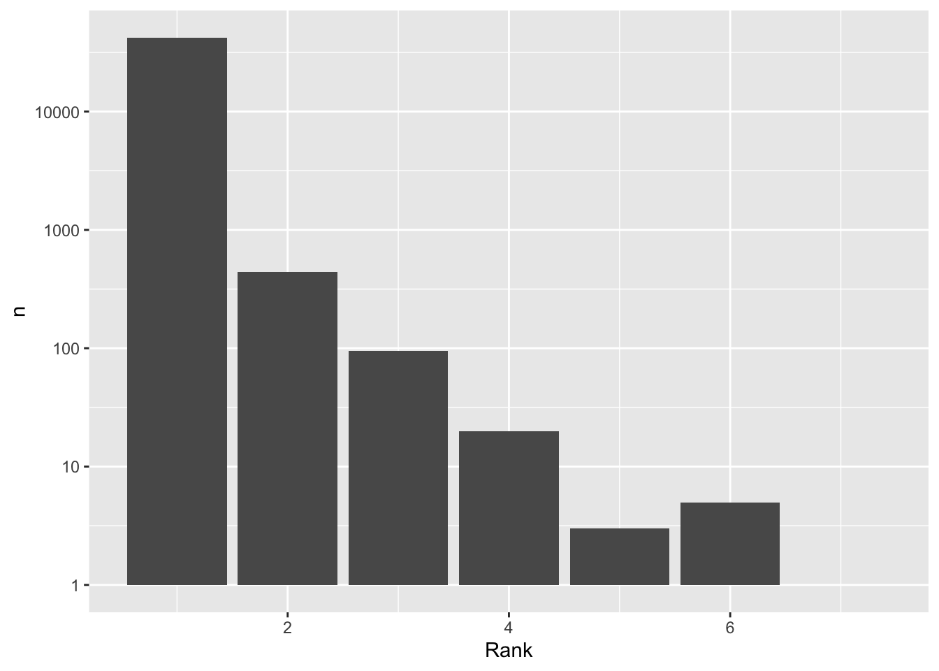
cc_qf[["psms_filtered"]] %>%
  rowData() %>%
  as_tibble() %>%
count(Search.Engine.Rank) %>%
ggplot(aes(Search.Engine.Rank, n)) +
geom_col() +
scale_y_log10() 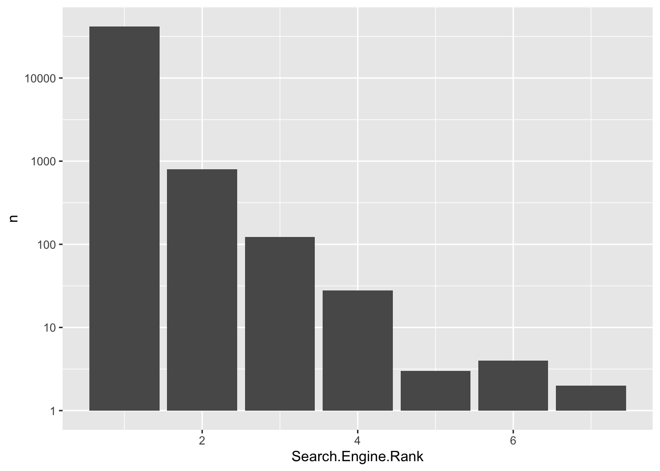
Part 2
Now let’s keep only PSMs with a rank of 1,
cc_qf <- cc_qf %>%
  filterFeatures(~ Rank == 1, i = "psms_filtered") %>%
  filterFeatures(~ Search.Engine.Rank == 1, i = "psms_filtered") %>%
  filterFeatures(~ PSM.Ambiguity == "Unambiguous", i = "psms_filtered")
'Rank' found in 2 out of 2 assay(s).'Search.Engine.Rank' found in 2 out of 2 assay(s).'PSM.Ambiguity' found in 2 out of 2 assay(s).## After filtering
cc_qfAn instance of class QFeatures (type: bulk) with 2 sets:
[1] psms_raw: SummarizedExperiment with 45803 rows and 10 columns
[2] psms_filtered: SummarizedExperiment with 41794 rows and 10 columns We now have 41794 PSMs.
In quantitative proteomics when thinking about what PSMs to consider for take forward for quantitation we consider PSM uniqueness. By definition uniqueness in this context refers to (i) PSMs corresponding to a single protein only, or it can also refer to (ii) PSMs that map to multiple proteins within a single protein group. This distinction is ultimately up to the user. We do not consider PSMs corresponding to razor and shared peptides as these are linked to multiple proteins across multiple protein groups.
In this workflow, the final grouping of peptides to proteins will be done based on master protein accession. Therefore, differential expression analysis will be based on protein groups, and we here consider unique as any PSM linked to only one protein group. This means removing PSMs where “Number.of.Protein.Groups” is not equal to 1.
cc_qf <- cc_qf %>%
  filterFeatures(~ Number.of.Protein.Groups == 1, i = "psms_filtered")
'Number.of.Protein.Groups' found in 2 out of 2 assay(s).## After filtering
cc_qfAn instance of class QFeatures (type: bulk) with 2 sets:
[1] psms_raw: SummarizedExperiment with 45803 rows and 10 columns
[2] psms_filtered: SummarizedExperiment with 40044 rows and 10 columns 3.2.2 Addititional quality control filters available for TMT data
As well as the completion of standard data cleaning steps which are common to all quantitative proteomics experiments (see above), different experimental methods are accompanied by additional data processing considerations. Although we cannot provide an extensive discussion of all methods, we will draw attention to three key quality control parameters to consider for our use-case TMT data.
- Average reporter ion signal-to-noise (S/N)
The quantitation of a TMT experiment is dependent upon the measurement of reporter ion signals from either the MS2 or MS3 spectra. Since reporter ion measurements derived from a small number of ions are more prone to stochastic ion effects and reduced quantitative accuracy, we want to remove PSMs that rely such quantitation to ensure high data quality. When using an Orbitrap analyser, the number of ions is proportional to the S/N ratio of a peak. Hence, removing PSMs that have a low S/N value acts as a proxy for removing low quality quantitation.
- Isolation interference (%)
Isolation interference occurs when multiple TMT-labelled precursor peptides are co-isolated within a single data acquisition window. All co-isolated peptides go on to be fragmented together and reporter ions from all peptides contribute to the reporter ion signal. Hence, quantification for the identified peptide becomes inaccurate. To minimise the co-isolation interference problem observed at MS2, MS3-based analysis can be used McAlister et al. (2014). Nevertheless, we remove PSMs with a high percentage isolation interference to prevent the inclusion of inaccurate quantitation values.
- Synchronous precursor selection mass matches (%) - SPS-MM
SPS-MM is a parameter unique to the Proteome Discoverer software which lets users quantify the percentage of MS3 fragments that can be explicitly traced back to the precursor peptides. This is important given that quantitation is based on the MS3 spectra.
Here we will apply the default quality control thresholds as suggested by Thermo Fisher and keep features with:
- Average reporter ion S/N >= 10
- Isolation interference < 75%
- SPS-MM >= 65%
We also remove features that do not have information regarding these quality control parameters i.e., have an NA value in the corresponding columns of the rowData. To remove these features we include the na.rm = TRUE argument.
cc_qf <- cc_qf %>%
  filterFeatures(~ Average.Reporter.SN >= 10,
                 na.rm = TRUE, i = "psms_filtered") %>%
  filterFeatures(~ Isolation.Interference.in.Percent <= 75,
                 na.rm = TRUE, i = "psms_filtered") %>%
  filterFeatures(~ SPS.Mass.Matches.in.Percent >= 65,
                 na.rm = TRUE, i = "psms_filtered")
'Average.Reporter.SN' found in 2 out of 2 assay(s).'Isolation.Interference.in.Percent' found in 2 out of 2 assay(s).'SPS.Mass.Matches.in.Percent' found in 2 out of 2 assay(s).In reality, we advise that users take a look at their data to decide whether the default quality control thresholds applied above are appropriate. If there is reason to believe that the raw MS data was of lower quality than desired, it may be sensible to apply stricter thresholds here. Similarly, if users wish to carry out a more stringent or exploratory analyses, these thresholds can be altered accordingly. For code and more information please see Hutchings et al. (2024).
3.2.3 Controlling false discovery rate (FDR)
The data cleaning steps that we have carried out so far have mainly been concerned with achieving high quality quantitation. However, we also want to be confident in our PSMs and their corresponding peptide and protein identifications.
To identify the peptides present in each of our samples we used a third party software to carry out a database search. Raw MS spectra are matched to theoretical spectra that are generated via in silico digestion of our desired protein database. The initial result of this search is a list of peptide spectrum matches, PSMs. A database search will identify PSMs for the majority of MS spectra, but only a minority of these will be true positives. In the same way that experiments must be conducted with controls, database search identifications need to be statistically validated to avoid false positives. The most widely used method for reducing the number of false positive identifications is to control the false discovery rate (FDR).
Target-decoy approach to FDR control
The most common approach to FDR control is the target-decoy approach. This involves searching the raw MS spectra against both a target and decoy database. The target database contains all protein sequences which could be in our sample (the human proteome and potential contaminants). The decoy database contains fake proteins that should not be present in the sample. For example, a decoy database may contain reversed or re-shuffled sequences. The main principle is that by carrying out these two searches we are able to estimate the the proportion of total PSMs that are false (matched to the decoy sequences) and apply score-based thresholding to shift this false discovery rate to a desired maximum. Typically expression proteomics utilises a maximum FDR of 0.01 or 0.05, that is to say 1% or 5% of PSMs are accepted false positives.
PSM level local FDR
The first FDR to be calculated is that for the PSMs themselves, often referred to as local FDR. As mentioned previously, each PSM is given a score indicating how likely it is to be correct or incorrect, depending on the search engine used. Based on these scores, each candidate PSM is ranked such that rank 1 PSMs have the highest probability of being correct or lowest probability of being incorrect. To calculate the local FDR for a PSM, the score for that PSM is taken as a threshold, and all PSMs with a score equal to or better than that PSM are extracted. The proportion of false positives within this population of PSMs is taken as its local FDR. In this way, the FDR can be thought of as the proportion of false positives above the critical score threshold.
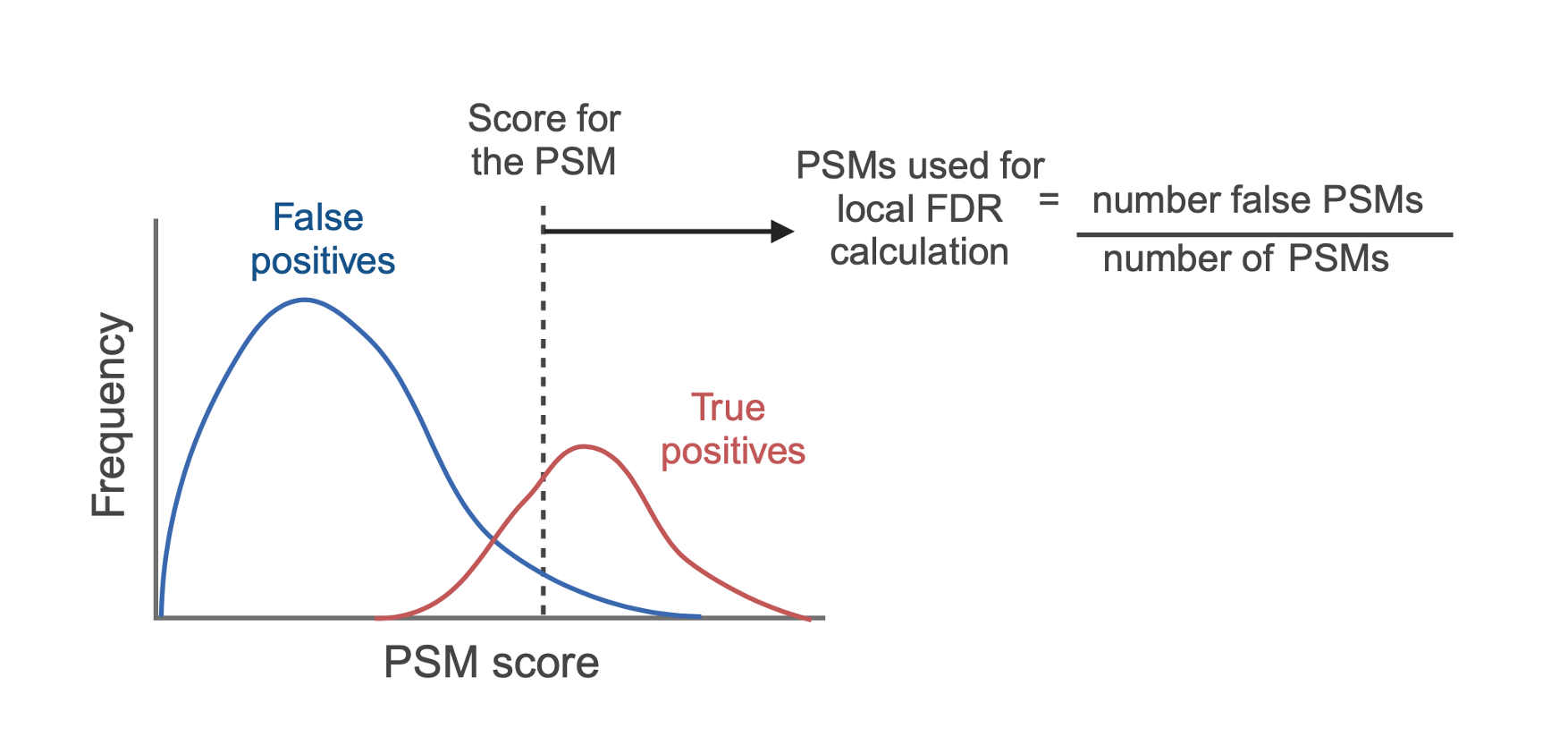
In the parameters for our identification search using Proteome Discoverer we specified a PSM level FDR threshold. We did this by allocating PSM confidence levels as ‘high’, ‘medium’ or ‘low’ depending on whether their FDR was < 0.01, < 0.05 or > 0.05. We then told Proteome Discoverer to only retain high confidence PSMs, those with a local FDR < 0.01. The local FDR indirectly tells us the probability of a PSM being a false positive, given the score it has.
Let’s double check that we only have high confidence PSMs.
cc_qf[["psms_raw"]] %>%
  rowData() %>%
  as_tibble() %>%
  pull(Confidence) %>%
  table()
.
High
45803 As expected, all of the PSMs in our data are of high confidence.
Protein level FDR thresholding is still required
Although we have already applied a PSM level FDR threshold to the data (during the identification search), it is highly recommended to set a protein level FDR threshold. This is because each peptide can have multiple PSMs and each protein can be supported by multiple peptides, thus resulting in the potential for amplification of the FDR during data aggregation. At a given PSM level score threshold, the peptide level FDR is greater than the PSM level FDR. Similarly, the protein level FDR is greater than the peptide level FDR.
To be absolutely confident in our final protein data we need to apply a protein level FDR. Unfortunately, third party software typically generates output tables in a sequential manner and there is currently no way to include information about the protein level FDR in the PSM level output. Therefore, we have to import the protein level output to get this information. The file is called cell_cycle_total_proteome_analysis_Proteins.txt.
We begin by using the read.delim function to read in the data,
## Applying protein level FDR - import protein output from database search
protein_data_PD <- read.delim(file = "data/cell_cycle_total_proteome_analysis_Proteins.txt")
Let’s check the dimensions of the protein level output,
dim(protein_data_PD)[1] 4904 72The output contains 4904 proteins. Let’s compare this to the number of master protein accessions in our raw and filtered PSM data,
## Number of master proteins in our raw data
cc_qf[["psms_raw"]] %>%
  rowData() %>%
  as_tibble() %>%
  pull(Master.Protein.Accessions) %>%
  unique() %>%
  length()
[1] 5267## Number of master proteins in our filtered data
cc_qf[["psms_filtered"]] %>%
rowData() %>%
as_tibble() %>%
pull(Master.Protein.Accessions) %>%
unique() %>%
length()[1] 3912It looks like the protein level output has fewer proteins than the raw PSM file but more proteins than our filtered PSM data. This tells us that Proteome Discoverer has done some filtering throughout the process of aggregating from PSM to peptide to protein, but not as much filtering as we have done manually in R. This makes sense because we did not set any quality control thresholds on co-isolation interference, reporter ion S/N ratio or SPS-MM during the search.
Now let’s look to see where information about the protein level FDR is stored.
names(protein_data_PD) %>%
  head(10)
[1] "Checked" "Tags"
[3] "Protein.FDR.Confidence.Combined" "Master"
[5] "Proteins.Unique.Sequence.ID" "Protein.Group.IDs"
[7] "Accession" "Description"
[9] "Sequence" "FASTA.Title.Lines" We have a column called "Protein.FDR.Confidence.Combined". Let’s add this information to our rowData of the psms_filtered set of our QFeatures object.
First let’s extract the rowData and convert it to a data.frame so we can make use of dplyr,
## Extract the rowData and convert to a data.frame
psm_data_QF <-
  cc_qf[["psms_filtered"]] %>%
  rowData() %>%
  as.data.frame()
Now let’s subset the protein_data_PD data to keep only accession and FDR information,
## Select only the Accession and FDR info
protein_data_PD <-
  protein_data_PD %>%
  select(Accession, Protein.FDR.Confidence.Combined)
Now let’s use dplyr and the left_join function to do the matching between the protein PD data and our PSM data for us. We need to specify how we join them so we need to specify the argument by = c("Master.Protein.Accessions" = "Accession") to tell R we wish to join the two datasets by their protein Accessions. Note, in the rowData of the QFeatures object we have "Master.Protein.Accessions" and in the PD protein data the column is just called "Accessions". Check with your own data the explicit naming of your data files as this will differ between third party softwares.
## Use left.join from dplyr to add the FDR data to PSM rowData data.frame
fdr_confidence <- left_join(x = psm_data_QF,
                            y = protein_data_PD,
                            by = c("Master.Protein.Accessions" = "Accession")) %>%
  pull("Protein.FDR.Confidence.Combined")
NoteJoining data.frames
Note: when using left_join we specify the argument by = c("Master.Protein.Accessions" = "Accession") (note the = equals sign between the names). This tells left_join we want to match join the two data.frames by matching accession numbers between the the Master.Protein.Accessions column in psm_data_QF and the column called Accession in the protein_data_PD data.
Now let’s add the FDR information back to the QFeatures object,
## Now add this data to the QF object
rowData(cc_qf[["psms_filtered"]])$Protein.FDR.Confidence <- fdr_confidence
Now we can print a table to see how many of the PSMs in our data were found to have a high confidence after protein level FDR calculations.
cc_qf[["psms_filtered"]] %>%
  rowData() %>%
  as_tibble() %>%
  pull(Protein.FDR.Confidence) %>%
  table()
.
High Low Medium
25699 5 84 Most of the PSMs in our data were found to originate from proteins with high confidence (FDR < 0.01 at protein level), but there are a few that are medium or low confidence. Even though we set a PSM level FDR threshold of 0.01, some of the resulting proteins still exceed this FDR due to amplification of error during aggregation.
We can now use the filterFeatures function to remove PSMs that do not have a Protein_Confidence of ‘High’.
cc_qf <- cc_qf %>%
  filterFeatures(~ Protein.FDR.Confidence == "High",
                 i = "psms_filtered")
'Protein.FDR.Confidence' found in 1 out of 2 assay(s).No filter applied to the following assay(s) because one or more
filtering variables are missing in the rowData: psms_raw. You can
control whether to remove or keep the features using the 'keep'
argument (see '?filterFeature').Notice, we see a message output to the terminal after running the function that telling us that Protein.FDR.Confidence was only found in 1 of our experiment assays and as such no filter was applied to the raw data. This is correct and expected.
cc_qf[["psms_filtered"]] %>%
  rowData %>%
  as_tibble %>%
  pull(Protein.FDR.Confidence) %>%
  table()
.
High
25699 For more information about how FDR values are calculated and used see Prieto and Vázquez (2019).
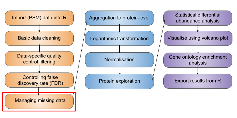
3.3 Management of missing data
Having cleaned our data, the next step is to deal with missing values. It is important to be aware that missing values can arise for different reasons in MS data, and these reasons determine the best way to deal with the missing data.
- Biological reasons - a peptide may be genuinely absent from a sample or have such low abundance that it is below the limit of MS detection
- Technical reasons - technical variation and the stochastic nature of MS (particularly using DDA) may lead to some peptides not being quantified. Some peptides have a lower ionization efficiency which makes them less compatible with MS analysis
Missing values that arise for different reasons can generally be deciphered by their pattern. For example, peptides that have missing quantitation values for biological reasons tend to be low intensity or completely absent peptides. Hence, these missing values are missing not at random (MNAR) and appear in an intensity-dependent pattern. By contrast, peptides that do not have quantitation due to technical reasons are missing completely at random (MCAR) and appear in an intensity-independent manner.
3.3.1 Influence of experimental design
All quantitative proteomics datasets will have some number of missing values, although the extent of data missingness differs between label-free and label-based DDA experiments as well as between DDA and DIA label-free experiments.
When carrying out a label-free DDA experiment, all samples are analysed via independent MS runs. Since the selection of precursor ions for fragmentation is somewhat stochastic in DDA (e.g., top N most abundant precursors are selected) experiments, different peptides may be identified and quantified across the different samples. In other words, not all peptides that are analysed in one sample will be analysed in the next, thus introducing a high proportion of missing values.
One of the advantages of using TMT labelling is the ability to multiplex samples into a single MS run. In the use-case, 10 samples were TMT labelled and pooled together prior to DDA MS analysis. As a result, the same peptides were quantified for all samples and we expect a lower proportion of missing values than if we were to use label-free DDA.
More recently, DIA MS analysis of label-free samples has increased in popularity. Here, instead of selecting a limited number of precursor peptides (typically the most abundance) for subsequent fragmentation and analysis, all precursors within a selected m/z window are selected. The analysis of all precursor ions within a defined range in every run results in more consistent coverage and accuracy than DDA experiments, hence lower missing values.
3.3.2 Exploration of missing data
The management of missing data can be considered in three main steps:
- Exploration of missing data - determine the number and pattern of missing values
- Removal of data with high levels of missingness - this could be features with missing values across too many samples or samples with an abnormally high proportion of missingness compared to the average
- Imputation (optional)
NoteEncoding of missing data
Before we begin managing the missing data, we first need to know what missing data looks like. In our data, missing values are notated as NA values. Alternative software may display missing values as being zero, or even infinite if normalisation has been applied during the database search. All functions used for the management of missing data within the QFeatures infrastructure use the NA notation. If we were dealing with a dataset that had an alternative encoding, we could apply the zeroIsNA() or infIsNA() functions to convert missing values into NA values.
The main function that facilitates the exploration of missing data in QFeatures is nNA. Let’s try to use this function. Again, we use the i = argument to specify which SummarizedExperiment within the QFeatures object that we wish to look at.
nNA(cc_qf, i = "psms_filtered")$nNA
DataFrame with 1 row and 3 columns
assay nNA pNA
<character> <integer> <numeric>
1 psms_filte... 14 5.44768e-05
$nNArows
DataFrame with 25699 rows and 4 columns
assay name nNA pNA
<character> <character> <integer> <numeric>
1 psms_filte... 7 0 0
2 psms_filte... 8 0 0
3 psms_filte... 9 0 0
4 psms_filte... 16 0 0
5 psms_filte... 18 0 0
... ... ... ... ...
25695 psms_filte... 45748 0 0
25696 psms_filte... 45752 0 0
25697 psms_filte... 45753 0 0
25698 psms_filte... 45777 0 0
25699 psms_filte... 45784 0 0
$nNAcols
DataFrame with 10 rows and 4 columns
assay name nNA pNA
<character> <character> <integer> <numeric>
1 psms_filte... Control 4 0.000155648
2 psms_filte... M_1 0 0.000000000
3 psms_filte... M_2 9 0.000350208
4 psms_filte... M_3 1 0.000038912
5 psms_filte... G1_1 0 0.000000000
6 psms_filte... G1_2 0 0.000000000
7 psms_filte... G1_3 0 0.000000000
8 psms_filte... DS_1 0 0.000000000
9 psms_filte... DS_2 0 0.000000000
10 psms_filte... DS_3 0 0.000000000The output from this function is a list of three DFrames. The first of these (called nNA) gives us information about missing data at the global level (i.e., for the entire SummarizedExperiment). We get information about the absolute number of missing values (nNA) and the proportion of the total data set that is missing values (pNA). The next two data frames also give us nNA and pNA but this time on a per row/feature (nNArows) and per column/sample (nNAcols) basis.
Let’s direct the output of nNA on each SummarizedExperiment to an object,
mv_raw <- nNA(cc_qf, i = "psms_raw")
mv_filtered <- nNA(cc_qf, i = "psms_filtered")
To access one DataFrame within a list we use the standard $ operator, followed by another $ operator if we wish to access specific columns.
Missing values down columns (sample) Print information regarding the number of missing values per column in the "mv_raw" data,
mv_raw$nNAcolsDataFrame with 10 rows and 4 columns
assay name nNA pNA
<character> <character> <integer> <numeric>
1 psms_raw Control 280 0.00611314
2 psms_raw M_1 161 0.00351505
3 psms_raw M_2 388 0.00847106
4 psms_raw M_3 177 0.00386438
5 psms_raw G1_1 118 0.00257625
6 psms_raw G1_2 123 0.00268541
7 psms_raw G1_3 88 0.00192127
8 psms_raw DS_1 116 0.00253259
9 psms_raw DS_2 143 0.00312207
10 psms_raw DS_3 110 0.00240159and after filtering,
mv_filtered$nNAcolsDataFrame with 10 rows and 4 columns
assay name nNA pNA
<character> <character> <integer> <numeric>
1 psms_filte... Control 4 0.000155648
2 psms_filte... M_1 0 0.000000000
3 psms_filte... M_2 9 0.000350208
4 psms_filte... M_3 1 0.000038912
5 psms_filte... G1_1 0 0.000000000
6 psms_filte... G1_2 0 0.000000000
7 psms_filte... G1_3 0 0.000000000
8 psms_filte... DS_1 0 0.000000000
9 psms_filte... DS_2 0 0.000000000
10 psms_filte... DS_3 0 0.000000000Now, we can extract the proportion of NAs in each sample,
mv_raw$nNAcols$pNA [1] 0.006113137 0.003515054 0.008471061 0.003864376 0.002576250 0.002685414
[7] 0.001921272 0.002532585 0.003122066 0.002401589We can also pass the output data from nNA to ggplot to visualise the missing data. This is particularly useful so that we can see whether any of our samples have an abnormally high proportion of missing values compared to the average. This could be the case if something had gone wrong during sample preparation. It is also useful to see whether there is any specific conditions that have a greater number of missing values.
In the following code chunk we visualise the proportion of missing values per sample and check for sample and condition bias.
In the raw data,
mv_raw$nNAcols %>%
  as_tibble() %>%
  mutate(condition = colData(cc_qf)$condition) %>%
  ggplot(aes(x = name, y = pNA, group = condition, fill = condition)) +
  geom_bar(stat = "identity") +
  labs(x = "Sample", y = "Proportion missing values") +
  theme_bw()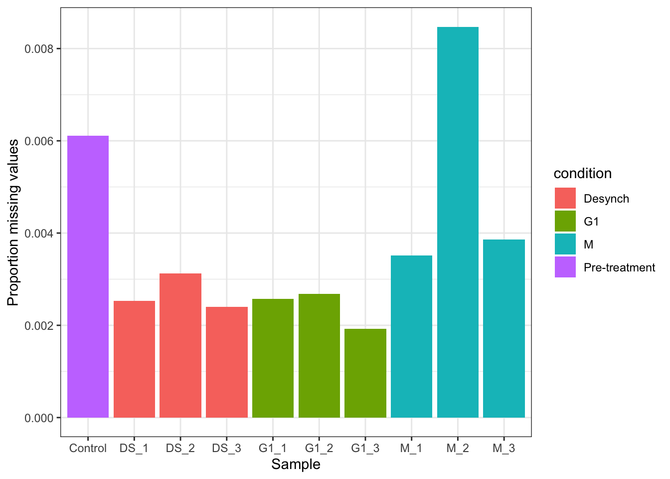
In the filtered data,
mv_filtered$nNAcols %>%
  as_tibble() %>%
  mutate(condition = colData(cc_qf)$condition) %>%
  ggplot(aes(x = name, y = pNA, group = condition, fill = condition)) +
  geom_bar(stat = "identity") +
  labs(x = "Sample", y = "Proportion missing values") +
  theme_bw()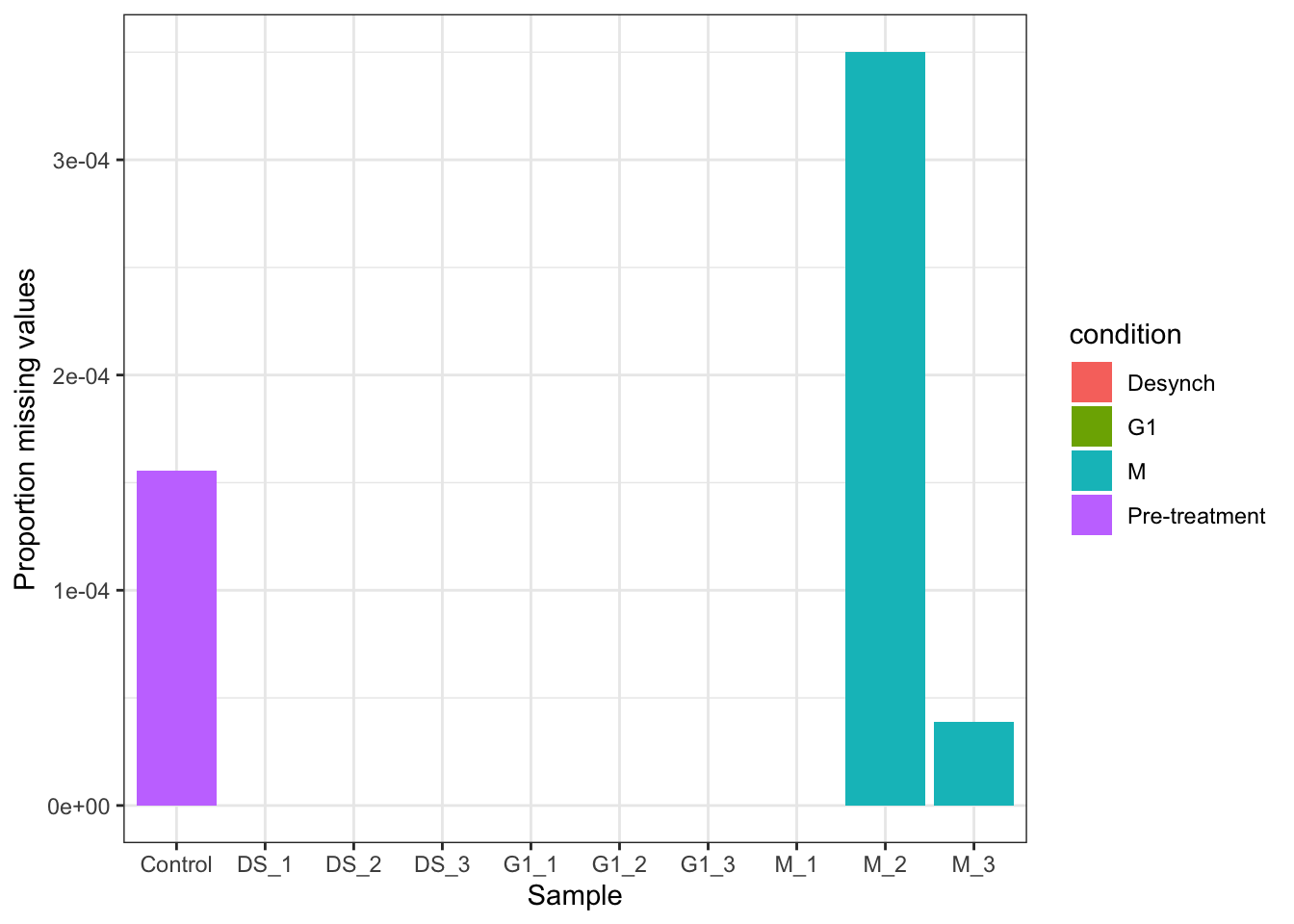
NoteMissing values - expectations
In this experiment we expect all samples to have a low proportion of missing values due to the TMT labelling strategy. We also expect that all samples should have a similar proportion of missing values because we do not expect cell cycle stage to have a large impact on the majority of the proteome. Hence, the samples here should be very similar. This is the case in most expression proteomics experiments which aim to identify differential protein abundance upon a cellular perturbation. However, in some other MS-based proteomics experiments this would not be the case. For example, proximity labelling and co-immunoprecipitation (Co-IP) experiments have control samples that are not expected to have any proteins in, although there is always a small amount of unwanted noise. In such cases it would be expected to have control samples with a large proportion of missing values and experimental samples with a much lower proportion. It is important to check that the data corresponds to the experimental setup.
Missing values across rows (PSMs) Print information regarding the number of missing values per row (PSM):
In the "psms_raw" data,
mv_raw$nNArowsDataFrame with 45803 rows and 4 columns
assay name nNA pNA
<character> <character> <integer> <numeric>
1 psms_raw 1 0 0.0
2 psms_raw 2 0 0.0
3 psms_raw 3 0 0.0
4 psms_raw 4 6 0.6
5 psms_raw 5 1 0.1
... ... ... ... ...
45799 psms_raw 45799 3 0.3
45800 psms_raw 45800 0 0.0
45801 psms_raw 45801 3 0.3
45802 psms_raw 45802 2 0.2
45803 psms_raw 45803 1 0.1The "psms_filtered" data,
mv_filtered$nNArowsDataFrame with 25699 rows and 4 columns
assay name nNA pNA
<character> <character> <integer> <numeric>
1 psms_filte... 7 0 0
2 psms_filte... 8 0 0
3 psms_filte... 9 0 0
4 psms_filte... 16 0 0
5 psms_filte... 18 0 0
... ... ... ... ...
25695 psms_filte... 45748 0 0
25696 psms_filte... 45752 0 0
25697 psms_filte... 45753 0 0
25698 psms_filte... 45777 0 0
25699 psms_filte... 45784 0 03.3.3 Removing data with high levels of missingness
Since the use-case data only has a small number of missing values, it makes sense to simply remove any PSM with a missing value. This is done using the filterNA function where the pNA argument specifies the maximum proportion of missing values to allow per feature.
cc_qf <- cc_qf %>%
  filterNA(pNA = 0, i = "psms_filtered")
Check that we now have no missing values,
nNA(cc_qf, i = "psms_filtered")$nNADataFrame with 1 row and 3 columns
assay nNA pNA
<character> <integer> <numeric>
1 psms_filte... 0 0We already established that none of our samples have an abnormally high proportion of missing values (relative to the average). Therefore, we do not need to remove any entire samples/columns.
3.3.4 Imputation of missing values
The final step when managing missing data is to consider whether to impute. Imputation involves the replacement of missing values with probable values. Unfortunately, estimating probable values is difficult and requires complex assumptions about why a value is missing. Given that imputation is difficult to get right and can have substantial effects on the results of downstream analysis, it is generally recommended to avoid it where we can. This means that if there is not a large proportion of missing values in our data, we should not impute. This is one of the reasons that it was easier in the use-case to simply remove the few missing values remaining so that we do not need to impute.
Unfortunately, not all datasets benefit from having so few missing values. Label-free proteomics experiments in particular have many more missing values than their label-based equivalents. For a more in-depth discussion of imputation and how to complete this within the QFeatures infrastructure, please see the Adapting this workflow to label-free proteomics data section.
TipKey Points
- The
filterFeaturesfunction can be used to remove data from aQFeaturesobject (or anSummarizedExperimentwithin aQFeaturesobject) based on filtering parameters within therowData. - Data processing includes (i) standard proteomics data cleaning steps e.g., removal of contaminants, and (ii) data-specific quality control filtering e.g., co-isolation interference thresholding for TMT data.
- The management of missing quantitative data in expression proteomics data is complex. The
nNAfunction can be used to explore missing data and thefilterNAfunction can be used to remove features with undesirably high levels of missing data. Where imputation is absolutely necessary, theimputefunction exists within theQFeaturesinfrastructure. - Protein level thresholding on false discovery rate is required to ensure confident identifications.
References
Frankenfield, Ashley M., Jiawei Ni, Mustafa Ahmed, and Ling Hao. 2022. “Protein Contaminants Matter: Building Universal Protein Contaminant Libraries for DDA and DIA Proteomics.” Journal of Proteome Research 21 (9): 2104–13. https://doi.org/10.1021/acs.jproteome.2c00145.
Hutchings, Charlotte, Charlotte S. Dawson, Thomas Krueger, Kathryn S. Lilley, and Lisa M. Breckels. 2024. “A Bioconductor Workflow for Processing, Evaluating, and Interpreting Expression Proteomics Data.” F1000Research 12 (September): 1402. https://doi.org/10.12688/f1000research.139116.2.
McAlister, Graeme C., David P. Nusinow, Mark P. Jedrychowski, et al. 2014. “MultiNotch MS3 Enables Accurate, Sensitive, and Multiplexed Detection of Differential Expression Across Cancer Cell Line Proteomes.” Analytical Chemistry 86 (14): 7150–58. https://doi.org/10.1021/ac502040v.
Prieto, Gorka, and Jesús Vázquez. 2019. “Calculation of False Discovery Rate for Peptide and Protein Identification.” In Methods in Molecular Biology. Springer New York. https://doi.org/10.1007/978-1-4939-9744-2_6.