2 Import and infrastructure

Learning Objectives

Understand the structure of SummarizedExperiment and QFeatures objects and how the two are related
Know how to import data into a QFeatures object
Demonstrate how to access information from each part of a QFeatures object by indexing and using assay, rowData and colData

2.1 The data structure

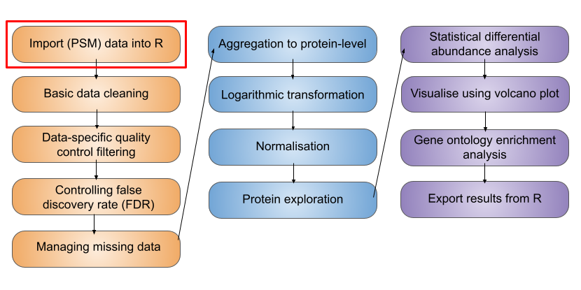
MS-based quantitative proteomics data is typically represented as a matrix in which the rows represent features (PSMs, peptides or proteins) and the columns contain information about these features, including their quantification measurements across several samples. As we saw before, this type of quantitative proteomics matrix can be generated by using third party softwares to process raw MS data. Moreover, the software usually outputs a quantitative matrix for each data level (e.g., PSM, peptide, peptide groups, protein groups). In this lesson we will explain how we can make use of R/Bioconductor packages with dedicated functions and data structures to store and manipulate quantitative proteomics data.

We begin with exporting our data at the lowest data-level. In this DDA TMT experiment this is the PSM level. This .txt file contains for every PSM identified the relative abundance of each PSMs across each sample as well as columns with PSM meta-data.

We will be using the Quantitative features for mass spectrometry, or QFeatures, Bioconductor package to import, store, and manipulate our data. Before we import the data into R using QFeatures it is first necessary to understand the structure of a QFeatures object and SummarizedExperiment object.

2.2 The structure of a `SummarizedExperiment`

To simplify the storage of quantitative proteomics data we can store the data as a SummarizedExperiment object (as shown in Figure 2.1).SummarizedExperiment objects can be conceptualised as data containers made up of three different parts:

The assay - a matrix which contains the quantitative data from a proteomics experiment. Each row represents a feature (a PSM, peptide or protein) and each column contains the quantitative data (measurements) from one experimental sample.
The rowData - a table (data frame) which contains all remaining information derived from an identification search (i.e. every column from your identification search output that was not a quantification column). Rows represent features but columns inform about different attributes of the feature (e.g., its sequence, name, modifications).
The colData - a table (data frame) to store sample metadata that would not appear in the output of your identification search. This could be for example, the cell line used, which condition, which replicate each sample corresponds to etc. Again, this information is stored in a matrix-like data structure.

Finally, there is also an additional container called metadata which is a place for users to store experimental metadata. For example, this could be which instrument the samples were run on, the operators name, the date the samples were run and so forth. We will focus on populating and understanding the above 3 main containers within a SummarizedExperiment.

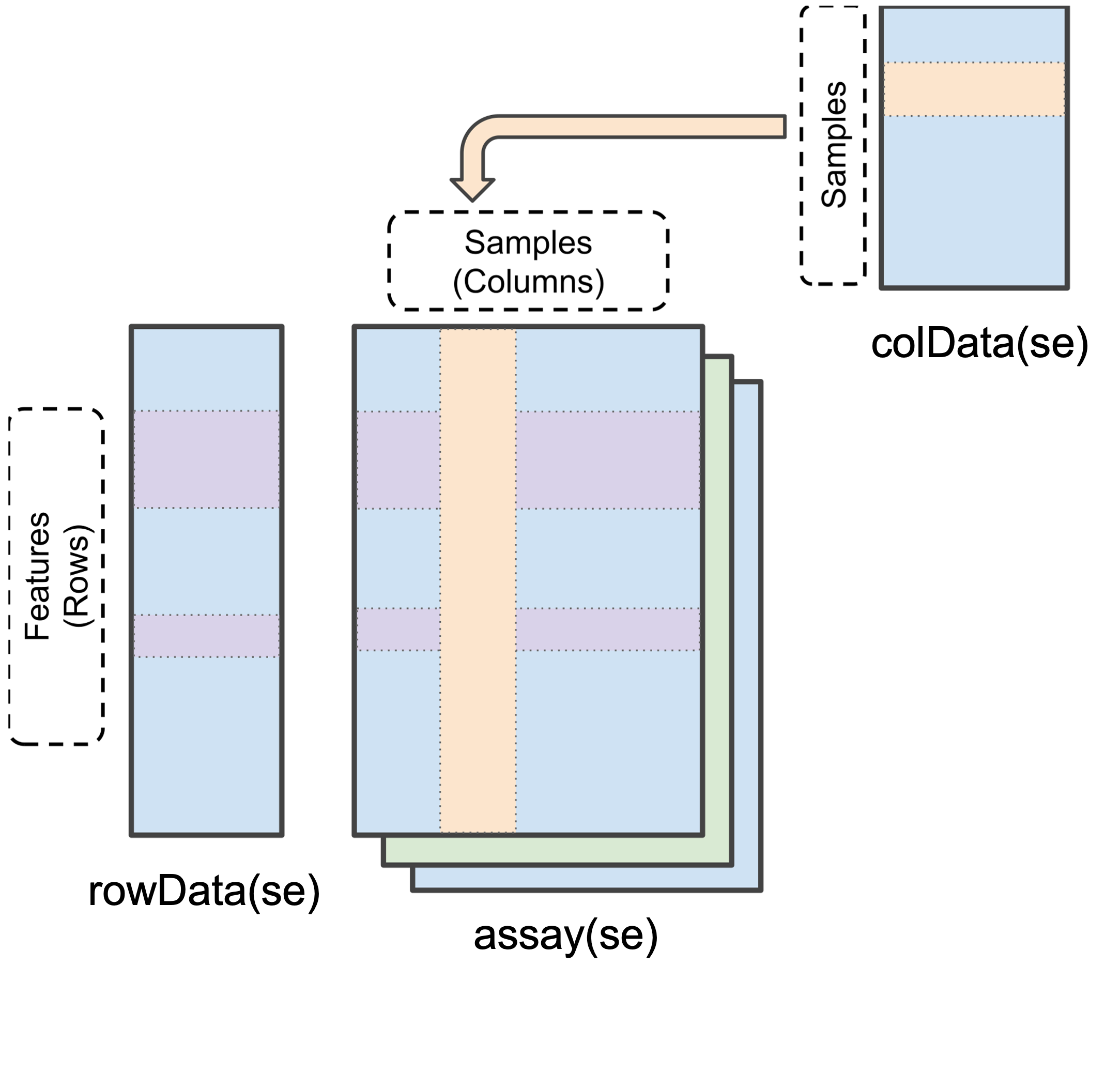
Figure 2.1: Diagramatic representation of the structure of a `SummarizedExperiment` object in R (modified from the SummarizedExperiment package)

Data stored in these three main areas can be easily accessed using the assay(), rowData() and colData() functions, as we will see later.

2.3 The structure of a `QFeatures` object

Whilst a SummarizedExperiment is able to neatly store quantitative proteomics data at a single data level (i.e., PSM, peptide or protein), a typical data analysis workflow requires us to look across multiple levels. For example, it is common to start an analysis with a lower data level and then aggregate upward towards a final protein-level dataset. Doing this allows for greater flexibility and understanding of the processes required to clean and aggregate the data.

A QFeatures object is essentially a list of SummarizedExperiment objects. However, the main benefit of using a QFeatures object over storing each data level as an independent SummarizedExperiment is that the QFeatures infrastructure maintains explicit links between the SummarizedExperiments that it stores. This allows for maximum traceability when processing data across multiple levels e.g., tracking which PSMs contribute to each peptide and which peptides contribute to a protein (Figure 2.2, modified from the QFeatures vignette with permission).

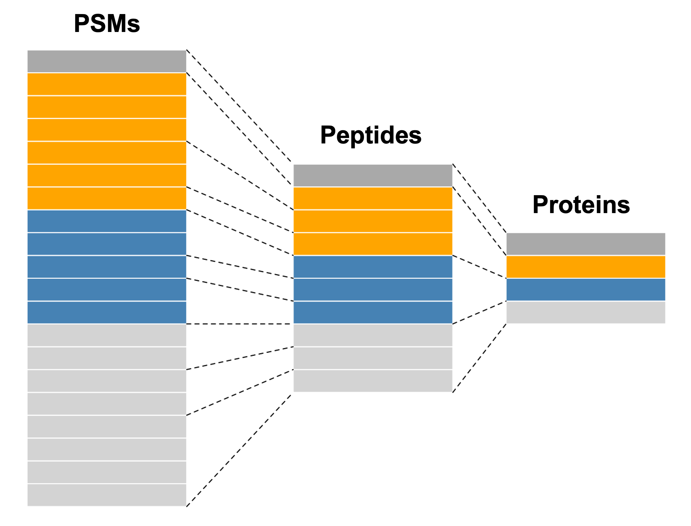
QFeatures

When talking about a QFeatures object, each dataset (individual SummarizedExperiment) can be referred to as an experiment. Previously, each dataset was referred to as an experimental assay, and some older resources may still use this term. However, the experimental assay should not be confused with the quantitative matrix section of a SummarizedExperiment, which is called the assay data.

In order to generate the explicit links between data levels, we need to import the lowest desired data level into a QFeatures object and aggregate upwards within the QFeatures infrastructure using the aggregateFeatures function, as we will later see in this course. If two SummarizedExperiments are generated separately and then added into the same QFeatures object, there will not automatically be links between them. In this case, if links are required, we can manually add links using the addAssayLink() function.

The best way to get our head around the QFeatures infrastructure is to import our data into a QFeatures object and start exploring.

2.4 Packages and working directory

During this course we will use several R/Bioconductor packages.

Let’s begin by opening RStudio and loading these packages into our working environment.

library("QFeatures")
library("limma")
library("factoextra")
library("org.Hs.eg.db")
library("clusterProfiler")
library("enrichplot")
library("patchwork")
library("tidyverse")
library("here")

Set your working directory to Course_Materials where you will find all the relevant data and R code files for this course. This can be achieved using the setwd function or by going to the menu Session -> Set Working Directory -> Choose Directory, in RStudio. Type list.files into your R console to check you can see the materials.

2.5 Importing data into R

There are several ways in which data can be imported into a QFeatures object. The most straightforward way is to first read the data into R as a data.frame using the read.delim function, and then import this data.frame into a QFeatures object.

Arguments to pass to readQFeatures:

assayData = A data.frame, or any object that can be coerced into a data.frame, holding the data
quantCols = an index for columns containing quantitative data. Can be a numeric index of the columns or a character vector containing the column names
name = name we want to give our first experiment, in the QFeatures object

Let’s read in the total proteome dataset from our experiment which is has been output from Proteome Discoverer at the PSM level. The file is called cell_cycle_total_proteome_analysis_PSMs.txt.

The first step is to read the data into R as a data.frame. We use the read.delim function.

df <- read.delim("data/cell_cycle_total_proteome_analysis_PSMs.txt")

Before we can create a QFeatures object we need to first identify which columns the quantitation data is stored in.

df %>% names()

 [1] "Checked"                           "Tags"                             
 [3] "Confidence"                        "Identifying.Node.Type"            
 [5] "Identifying.Node"                  "Search.ID"                        
 [7] "Identifying.Node.No"               "PSM.Ambiguity"                    
 [9] "Sequence"                          "Annotated.Sequence"               
[11] "Modifications"                     "Number.of.Proteins"               
[13] "Master.Protein.Accessions"         "Master.Protein.Descriptions"      
[15] "Protein.Accessions"                "Protein.Descriptions"             
[17] "Number.of.Missed.Cleavages"        "Charge"                           
[19] "Original.Precursor.Charge"         "Delta.Score"                      
[21] "Delta.Cn"                          "Rank"                             
[23] "Search.Engine.Rank"                "Concatenated.Rank"                
[25] "mz.in.Da"                          "MHplus.in.Da"                     
[27] "Theo.MHplus.in.Da"                 "Delta.M.in.ppm"                   
[29] "Delta.mz.in.Da"                    "Ions.Matched"                     
[31] "Matched.Ions"                      "Total.Ions"                       
[33] "Intensity"                         "Activation.Type"                  
[35] "NCE.in.Percent"                    "MS.Order"                         
[37] "Isolation.Interference.in.Percent" "SPS.Mass.Matches.in.Percent"      
[39] "Average.Reporter.SN"               "Ion.Inject.Time.in.ms"            
[41] "RT.in.min"                         "First.Scan"                       
[43] "Last.Scan"                         "Master.Scans"                     
[45] "Spectrum.File"                     "File.ID"                          
[47] "Abundance.126"                     "Abundance.127N"                   
[49] "Abundance.127C"                    "Abundance.128N"                   
[51] "Abundance.128C"                    "Abundance.129N"                   
[53] "Abundance.129C"                    "Abundance.130N"                   
[55] "Abundance.130C"                    "Abundance.131"                    
[57] "Quan.Info"                         "Peptides.Matched"                 
[59] "XCorr"                             "Number.of.Protein.Groups"         
[61] "Contaminant"                       "Percolator.q.Value"               
[63] "Percolator.PEP"                    "Percolator.SVMScore"

We can see the quantitation data is located in columns 47 - 56 which start with “Abundance…” followed by the identifying TMT tag. Naming of the abundance columns is dependent on the third party software used and version, please make sure you check you identify the relevant column numbers containing the quantitation data in your own data.

We will pass this information to the quantCols argument when we use the readQFeatures function. As this is the first data import before any processing so let’s call this data level "psms_raw".

## Import data into QF object
cc_qf <- readQFeatures(assayData = df,
                       quantCols = 47:56, 
                       name = "psms_raw")

Checking arguments.

Loading data as a 'SummarizedExperiment' object.

Formatting sample annotations (colData).

Formatting data as a 'QFeatures' object.

Finding help files

During this course we see many new functions. For more information on any R function type ? and the name of the function in the R console to bring up the relevant documentation. Or go to the Help menu in RStudio and Help -> Search R Help. For example, to see the help files and documentation for the readQFeatures function type ?readQFeatures in your RStudio console. The help documentation highlights what structure the input data should be (a vector, dataframe or matrix etc.) as well as which arguments are required or optional. When using more complex functions, such as those which we will use for statistical analysis, it is advisable to consult the help documentation to ensure that you understand what the function’s default parameters are. This will help you to make sure that the function does what you are expecting it to do.

2.6 Accessing information within a `QFeatures` object

Let’s take a look at our newly created object.

cc_qf

An instance of class QFeatures containing 1 assays:
 [1] psms_raw: SummarizedExperiment with 45803 rows and 10 columns

We see that we have created a QFeatures object containing a single SummarizedExperiment called “psms_raw”. There are 45803 rows in the data, representing 45803 PSMs. We also see that there are 10 columns representing our 10 samples.

We can access individual SummarizedExperiments within a QFeatures object using standard double bracket nomenclature (this is how you would normally access items of a list in R). As with all indexing we can use the list position or assay name.

## Indexing using position
cc_qf[[1]]

class: SummarizedExperiment 
dim: 45803 10 
metadata(0):
assays(1): ''
rownames(45803): 1 2 ... 45802 45803
rowData names(54): Checked Tags ... Percolator.PEP Percolator.SVMScore
colnames(10): Abundance.126 Abundance.127N ... Abundance.130C
  Abundance.131
colData names(0):

## Indexing using name
cc_qf[["psms_raw"]]

class: SummarizedExperiment 
dim: 45803 10 
metadata(0):
assays(1): ''
rownames(45803): 1 2 ... 45802 45803
rowData names(54): Checked Tags ... Percolator.PEP Percolator.SVMScore
colnames(10): Abundance.126 Abundance.127N ... Abundance.130C
  Abundance.131
colData names(0):

Within each SummarizedExperiment(SE), the rowData, colData and assay data are accessed using rowData(), colData() and assay(), respectively. Let’s use these functions to explore the data structure further.

2.6.1 The `assay` container

Let’s start with the quantitation data of our SE called psms_raw. This is stored in the assay slot.

assay(cc_qf[["psms_raw"]])

You will see that the R console is populated with the quantitation data and the whole dataset is too big to print to the screen. Let’s use the head command to show only the 6 lines (default) of the quantitation data.

Type into your R console,

head(assay(cc_qf[["psms_raw"]]))

  Abundance.126 Abundance.127N Abundance.127C Abundance.128N Abundance.128C
1          22.3           48.6           15.1           26.8           39.0
2          19.8           31.3           14.1           19.5           32.1
3           2.4            7.9            1.2            2.3            4.1
4           2.2             NA             NA             NA             NA
5           2.2            4.2            2.2            1.6            5.7
6            NA            1.7             NA             NA             NA
  Abundance.129N Abundance.129C Abundance.130N Abundance.130C Abundance.131
1           21.6           41.6           38.7           21.2          34.7
2           29.2           37.1           41.2           30.0          34.9
3            1.0            3.6            7.0            3.1           2.7
4            2.3            3.1             NA            1.7            NA
5            1.4             NA            3.6            4.0           4.0
6             NA             NA             NA             NA           2.7

This is equivalent to,

cc_qf[["psms_raw"]] %>% 
  assay() %>% 
  head()

  Abundance.126 Abundance.127N Abundance.127C Abundance.128N Abundance.128C
1          22.3           48.6           15.1           26.8           39.0
2          19.8           31.3           14.1           19.5           32.1
3           2.4            7.9            1.2            2.3            4.1
4           2.2             NA             NA             NA             NA
5           2.2            4.2            2.2            1.6            5.7
6            NA            1.7             NA             NA             NA
  Abundance.129N Abundance.129C Abundance.130N Abundance.130C Abundance.131
1           21.6           41.6           38.7           21.2          34.7
2           29.2           37.1           41.2           30.0          34.9
3            1.0            3.6            7.0            3.1           2.7
4            2.3            3.1             NA            1.7            NA
5            1.4             NA            3.6            4.0           4.0
6             NA             NA             NA             NA           2.7

The first code chunk uses nested functions and the second uses pipes. Throughout this course for ease of coding and clarity we will use pipes and where appropriate follow the tidyverse style of coding for clarity.

The dplyr pipe

In this course we will frequently use pipes, specifically the dplyr pipe part of the dplyr package and tidyverse. The pipe operator allows you to chain together multiple operations and code complex tasks in a more linear and understandable way, rather than having to nest multiple function calls or write multiple lines of code. For more information see Hadley Wickham’s Tidyverse at https://www.tidyverse.org.

Challenge 1: Accessing information

Level:

Explore the QFeatures object you have just created.

How many experimental assays do we currently have in the object?
How many PSMs have been identified in the data?
How do you access and view the quantitation data i.e. the relative abundance of each PSM across the samples?

Answer

Task 1

When we type the name of the the object cc_qf a summary of the data is printed to the screen. This summary shows us a summary of the number of experimental assays we have in the data.

cc_qf

An instance of class QFeatures containing 1 assays:
 [1] psms_raw: SummarizedExperiment with 45803 rows and 10 columns

Since a QFeatures object is a list of SummarizedExperiment objects, we can use length(cc_qf) to check how many objects we have inside it

length(cc_qf)

[1] 1

Alternatively, we can also extract the list of experiments directly using

experiments(cc_qf)

ExperimentList class object of length 1:
 [1] psms_raw: SummarizedExperiment with 45803 rows and 10 columns

Task 2

Similarly, the object summary also tells us the number of PSMs. We can also extract the number of rows (PSMs in our case) for a given level (i.e. psms_raw)

cc_qf[["psms_raw"]] %>% 
  nrow()

[1] 45803

Task 3

We can use the assay accessor,

cc_qf[["psms_raw"]] %>% 
  assay()

or equivalently,

assay(cc_qf[["psms_raw"]])

As expected, the assay slot contains 10 quantitative columns corresponding to the 10 samples in our experiment. We see some quantitative values and some missing values, here denotated NA.

2.6.2 The `rowData` container

Now let’s examine the the rowData slot,

cc_qf[["psms_raw"]] %>%
  rowData() %>%
  names()

 [1] "Checked"                           "Tags"                             
 [3] "Confidence"                        "Identifying.Node.Type"            
 [5] "Identifying.Node"                  "Search.ID"                        
 [7] "Identifying.Node.No"               "PSM.Ambiguity"                    
 [9] "Sequence"                          "Annotated.Sequence"               
[11] "Modifications"                     "Number.of.Proteins"               
[13] "Master.Protein.Accessions"         "Master.Protein.Descriptions"      
[15] "Protein.Accessions"                "Protein.Descriptions"             
[17] "Number.of.Missed.Cleavages"        "Charge"                           
[19] "Original.Precursor.Charge"         "Delta.Score"                      
[21] "Delta.Cn"                          "Rank"                             
[23] "Search.Engine.Rank"                "Concatenated.Rank"                
[25] "mz.in.Da"                          "MHplus.in.Da"                     
[27] "Theo.MHplus.in.Da"                 "Delta.M.in.ppm"                   
[29] "Delta.mz.in.Da"                    "Ions.Matched"                     
[31] "Matched.Ions"                      "Total.Ions"                       
[33] "Intensity"                         "Activation.Type"                  
[35] "NCE.in.Percent"                    "MS.Order"                         
[37] "Isolation.Interference.in.Percent" "SPS.Mass.Matches.in.Percent"      
[39] "Average.Reporter.SN"               "Ion.Inject.Time.in.ms"            
[41] "RT.in.min"                         "First.Scan"                       
[43] "Last.Scan"                         "Master.Scans"                     
[45] "Spectrum.File"                     "File.ID"                          
[47] "Quan.Info"                         "Peptides.Matched"                 
[49] "XCorr"                             "Number.of.Protein.Groups"         
[51] "Contaminant"                       "Percolator.q.Value"               
[53] "Percolator.PEP"                    "Percolator.SVMScore"

The columns of our rowData contain non-quantitative information derived from the third party identification search. The exact names of variables will differ between software and change over time, but the key information that we need to know about each feature (here PSMs) will always be here.

This information includes the sequence of the peptide to which each PSM corresponds ("Sequence") as well as the master protein to which the peptide is assigned ("Master.Protein.Accessions"). We will come across more of the variables stored in the rowData when we come to data cleaning and filtering.

We again use the head command to print the first 6 rows of the rowData

cc_qf[["psms_raw"]] %>%
  rowData() %>%
  head()

DataFrame with 6 rows and 54 columns
      Checked      Tags  Confidence Identifying.Node.Type Identifying.Node
  <character> <logical> <character>           <character>      <character>
1       False        NA        High            Sequest HT    Sequest HT...
2       False        NA        High            Sequest HT    Sequest HT...
3       False        NA        High            Sequest HT    Sequest HT...
4       False        NA        High            Sequest HT    Sequest HT...
5       False        NA        High            Sequest HT    Sequest HT...
6       False        NA        High            Sequest HT    Sequest HT...
    Search.ID Identifying.Node.No PSM.Ambiguity      Sequence
  <character>           <integer>   <character>   <character>
1           A                   2 Unambiguou...        REEEMR
2           A                   2 Unambiguou...     QQNGTASSR
3           A                   2 Unambiguou...      CHMEENQR
4           A                   2 Unambiguou...        QACQER
5           A                   2 Unambiguou...     HSEAATAQR
6           A                   2 Unambiguou... QQQQQQQHQQ...
  Annotated.Sequence Modifications Number.of.Proteins Master.Protein.Accessions
         <character>   <character>          <integer>               <character>
1             rEEEmR N-Term(TMT...                  2             P49755; Q1...
2          qQnGTASSR N-Term(TMT...                  1                    Q92917
3           cHmEENQR N-Term(TMT...                  1                    Q96TC7
4             qAcQER N-Term(TMT...                  1                    P26358
5          hSEAATAQR N-Term(TMT...                  1                    Q14103
6      qQQQQQQHQQ... N-Term(TMT...                  1                    Q6Y7W6
  Master.Protein.Descriptions Protein.Accessions Protein.Descriptions
                  <character>        <character>          <character>
1               Transmembr...      P49755; Q1...        Transmembr...
2               G-patch do...             Q92917        G-patch do...
3               Regulator ...             Q96TC7        Regulator ...
4               DNA (cytos...             P26358        DNA (cytos...
5               Heterogene...             Q14103        Heterogene...
6               GRB10-inte...             Q6Y7W6        GRB10-inte...
  Number.of.Missed.Cleavages    Charge Original.Precursor.Charge Delta.Score
                   <integer> <integer>                 <integer>   <numeric>
1                          1         2                         2      0.1696
2                          0         2                         2      0.1154
3                          0         3                         3      1.0000
4                          0         2                         2      0.2849
5                          0         2                         2      0.4780
6                          0         3                         3      0.4098
   Delta.Cn      Rank Search.Engine.Rank Concatenated.Rank  mz.in.Da
  <numeric> <integer>          <integer>         <integer> <numeric>
1         0         1                  1                 3   547.776
2         0         1                  1                 1   589.802
3         0         1                  1                 1   450.202
4         0         1                  1                 1   510.758
5         0         1                  1                 1   600.320
6         0         1                  1                 1   635.659
  MHplus.in.Da Theo.MHplus.in.Da Delta.M.in.ppm Delta.mz.in.Da Ions.Matched
     <numeric>         <numeric>      <numeric>      <numeric>  <character>
1      1094.55           1094.55          -0.99       -0.00054          0/0
2      1178.60           1178.60           0.06        0.00003          0/0
3      1348.59           1348.59          -1.08       -0.00049          0/0
4      1020.51           1020.51          -1.44       -0.00074          0/0
5      1199.63           1199.63          -0.33       -0.00020          0/0
6      1904.96           1904.96          -1.33       -0.00084          0/0
  Matched.Ions Total.Ions Intensity Activation.Type NCE.in.Percent    MS.Order
     <integer>  <integer> <numeric>     <character>      <numeric> <character>
1            0          0  505446.3             CID             NA         MS2
2            0          0  197059.8             CID             NA         MS2
3            0          0   76685.6             CID             NA         MS2
4            0          0  103765.7             CID             NA         MS2
5            0          0  238514.8             CID             NA         MS2
6            0          0   76203.7             CID             NA         MS2
  Isolation.Interference.in.Percent SPS.Mass.Matches.in.Percent
                          <numeric>                   <integer>
1                           0.00000                          50
2                          47.04837                          50
3                          30.96584                          50
4                           3.10827                          60
5                          12.56510                          70
6                           0.00000                          80
  Average.Reporter.SN Ion.Inject.Time.in.ms RT.in.min First.Scan Last.Scan
            <numeric>             <numeric> <numeric>  <integer> <integer>
1                30.8                    60   39.4997       5816      5816
2                28.7                    60   39.8252       5902      5902
3                 3.5                    60   40.0773       5967      5967
4                 0.9                    60   40.3077       6035      6035
5                 2.8                    60   40.7688       6151      6151
6                 0.4                    60   40.8788       6183      6183
  Master.Scans Spectrum.File     File.ID Quan.Info Peptides.Matched     XCorr
     <integer>   <character> <character> <logical>        <integer> <numeric>
1         5810 NocArrest_...        F1.1        NA              104      1.71
2         5898 NocArrest_...        F1.1        NA              125      1.82
3         5961 NocArrest_...        F1.1        NA                4      0.94
4         6031 NocArrest_...        F1.1        NA              105      1.86
5         6147 NocArrest_...        F1.1        NA              136      1.82
6         6177 NocArrest_...        F1.1        NA              285      1.22
  Number.of.Protein.Groups Contaminant Percolator.q.Value Percolator.PEP
                 <integer> <character>          <numeric>      <numeric>
1                        2       False          0.0033430       0.030030
2                        1       False          0.0009278       0.006729
3                        1       False          0.0014400       0.012330
4                        1       False          0.0009278       0.006435
5                        1       False          0.0004399       0.002259
6                        1       False          0.0006928       0.003668
  Percolator.SVMScore
            <numeric>
1               0.132
2               0.352
3               0.260
4               0.360
5               0.536
6               0.453

Challenge 2: Calculating the number of peptides and proteins in our dataset

Level:

Explore the information stored in the rowData from the Proteome Discoverer search. Look at the first few rows of this data matrix by using the head function and find a column that related to the peptide sequence information.

What class is the rowData container? How many rows and columns are in this data structure?
Extract the rowData and convert it to a tibble or data.frame. Find a column that contains information that relates to the peptide sequence. Pull this information and calculate how many unique peptide sequences we have in the dataset.

Hint

Using the unique function may be helpful.

How many protein groups (master proteins) have been identified in the dataset?

Hint

Again, convert the rowData to a tibble or data.frame and find a column that contains information that relates to protein identification.

Answer

Task 1

cc_qf[["psms_raw"]] %>% 
  rowData() %>% 
  class()

[1] "DFrame"
attr(,"package")
[1] "S4Vectors"

We see that the rowData is of class "DFrame". This is a type of data frame. Will will convert this to a data.frame or tibble throughout this couse to make use of tidyverse functions.

cc_qf[["psms_raw"]] %>% 
  rowData() %>% 
  dim()

[1] 45803    54

We see we have 45803 PSMs and 54 columns of information relating to each PSM.

Task 2

There are many ways to extract the number of peptides from our datasets. The current data level shows the total number of PSMs (peptide spectrum matches). Although PSMs are fragments of identified peptide sequences, there can be many PSMs per unique peptide. The rowData is where we have stored information relating to our samples that are not quantitation data. The column Sequence contains the peptide sequence from which the PSM is is derived.

In the following lines of code we, - Extract the rowData - Convert the rowData which is DFrame to either a data.frame or tibble. We could use the as.data.frame or as_tibble functions, respectively, which we will allow us to use pipes. - Extract the column Sequence. - Use the unique function to group together PSMs from the same peptide. - Finally, we use the length command to count the number of peptides.

## Using pipes
cc_qf[["psms_raw"]] %>%
  rowData() %>%
  as_tibble() %>%
  pull(Sequence) %>%
  unique() %>%
  length()

[1] 26738

Alternative solution (among many others)

## Without pipes
rd <- rowData(cc_qf[["psms_raw"]])
tbl <- unique(rd$Sequence) 
length(tbl)

[1] 26738

We have 26738 peptides.

Task 3

Information regarding the protein groups is found in the Master.Protein.Accessions column.

## Using pipes
cc_qf[["psms_raw"]] %>%
  rowData() %>%
  as_tibble() %>%
  pull(Master.Protein.Accessions) %>%
  unique() %>%
  length()

[1] 5267

Alternative solution (among many others)

## Without pipes
tbl <- unique(rd$Master.Protein.Accessions) 
length(tbl)

[1] 5267

We have 5267 protein groups represented by 5267 master proteins.

2.6.3 The `colData` container

The final slot within our SummarizedExperiment is the colData.

cc_qf[["psms_raw"]] %>%
  colData()

DataFrame with 10 rows and 0 columns

We see this is also a DataFrame structure.

cc_qf[["psms_raw"]] %>%
  colData() %>% 
  class()

[1] "DFrame"
attr(,"package")
[1] "S4Vectors"

It has 10 rows, one per sample, but no columns yet. This is because the sample metadata is not derived from an identification search and does not appear in our output .txt file. If we want to store extra information about our samples, we need to add this to the colData ourselves.

Each row of this 10 by 0 DataFrame corresponds to some feature of the quantitation channel. The names of these rows are the TMT sample names,

cc_qf[["psms_raw"]] %>%
  colData() %>% 
  rownames()

 [1] "Abundance.126"  "Abundance.127N" "Abundance.127C" "Abundance.128N"
 [5] "Abundance.128C" "Abundance.129N" "Abundance.129C" "Abundance.130N"
 [9] "Abundance.130C" "Abundance.131"

2.6.4 Annotating samples by adding meta-data

The colData contains information about the samples. We can create a data.frame in R with information regarding the samples, replicates, conditions and TMT tag used or we can read in this information into R from a spreadsheet or .csv.

Let’s open the file coldata.csv and then read it into R and add it to our QFeatures object.

## Read in coldata .csv
metadata_df <- read.csv("data/samples_meta_data.csv")

## View data
metadata_df

                X  sample rep     condition  tag
1   Abundance.126 Control  NA Pre-treatment  126
2  Abundance.127N     M_1   1             M 127N
3  Abundance.127C     M_2   2             M 127C
4  Abundance.128N     M_3   3             M 128N
5  Abundance.128C    G1_1   1            G1 128C
6  Abundance.129N    G1_2   2            G1 129N
7  Abundance.129C    G1_3   3            G1 129C
8  Abundance.130N    DS_1   1       Desynch 130N
9  Abundance.130C    DS_2   2       Desynch 130C
10  Abundance.131    DS_3   3       Desynch  131

This .csv file has 10 rows, importantly the rows are annotated using the names of the rowData of our object, e.g. “Abundance.126”, “Abundance.127N” etc.

We can add information from this .csv to our colData

## Annotate colData with condition information
cc_qf$sample <- metadata_df$sample

## Now add replicate information
cc_qf$rep <- metadata_df$rep

## And condition information
cc_qf$condition <- metadata_df$condition

## Add the TMT information
cc_qf$tag <- metadata_df$tag

## Verify
colData(cc_qf)

DataFrame with 10 rows and 4 columns
                    sample       rep     condition         tag
               <character> <integer>   <character> <character>
Abundance.126      Control        NA Pre-treatm...         126
Abundance.127N         M_1         1             M        127N
Abundance.127C         M_2         2             M        127C
Abundance.128N         M_3         3             M        128N
Abundance.128C        G1_1         1            G1        128C
Abundance.129N        G1_2         2            G1        129N
Abundance.129C        G1_3         3            G1        129C
Abundance.130N        DS_1         1       Desynch        130N
Abundance.130C        DS_2         2       Desynch        130C
Abundance.131         DS_3         3       Desynch         131

## Apply this to the first assay so that it is carried up
colData(cc_qf[["psms_raw"]]) <- colData(cc_qf)

We can also change the names of our samples to simplify our downstream coding as well as our visualisation. This is done by changing the colnames.

 ## Change col names to represent the sample
colnames(cc_qf[["psms_raw"]]) <- cc_qf$sample

## Verify
colData(cc_qf[["psms_raw"]])

DataFrame with 10 rows and 4 columns
             sample       rep     condition         tag
        <character> <integer>   <character> <character>
Control     Control        NA Pre-treatm...         126
M_1             M_1         1             M        127N
M_2             M_2         2             M        127C
M_3             M_3         3             M        128N
G1_1           G1_1         1            G1        128C
G1_2           G1_2         2            G1        129N
G1_3           G1_3         3            G1        129C
DS_1           DS_1         1       Desynch        130N
DS_2           DS_2         2       Desynch        130C
DS_3           DS_3         3       Desynch         131

Challenge 3: Miscleavages

Level:

One of the pieces of information given by the Proteome Discoverer software used to produce the TMT data is the number of missed cleavages. This is stored in a rowData column named "Number.of.Missed.Cleavages". Can you count how many occurrences of missed cleavages there are in our data?

Answer

cc_qf[["psms_raw"]] %>%
  rowData() %>%
  as_tibble() %>%
  count(Number.of.Missed.Cleavages)

# A tibble: 3 × 2
  Number.of.Missed.Cleavages     n
                       <int> <int>
1                          0 34988
2                          1  9709
3                          2  1106

We see that during the identification search missed cleavages were limited to a maximum of 2 missed cleavage sites. This is typical in bottom-up proteomics.

Key Points

The QFeatures infrastructure provides a convenient and transparent way to store proteomics data across multiple levels.
A QFeatures object stores each data level as a SummarizedExperiment, also called an experimental assay, with explicit links maintained between features across different experimental assays (e.g., links between all PSMs contributing to a peptide).
Explicit links between experimental assays are (i) generated automatically when aggregating data using aggregateFeatures or (ii) added manually using the addAssayLinks function, as we will see later on.
Within each SummarizedExperiment the feature data is stored within the rowData, quantitative data in the assay, and sample metadata in the colData. These slots are accessible using their corresponding functions.

2.1 The data structure

2.2 The structure of a SummarizedExperiment

2.3 The structure of a QFeatures object

2.4 Packages and working directory

2.5 Importing data into R

2.6 Accessing information within a QFeatures object

2.6.1 The assay container

2.6.2 The rowData container

2.6.3 The colData container

2.6.4 Annotating samples by adding meta-data

References

2.2 The structure of a `SummarizedExperiment`

2.3 The structure of a `QFeatures` object

2.6 Accessing information within a `QFeatures` object

2.6.1 The `assay` container

2.6.2 The `rowData` container

2.6.3 The `colData` container