TMT QC PSM-level quantification and summarisation to protein-level abundance
Tom Smith
2024-07-01
TMT_PSM_QC_Summarisation.RmdQuantitative proteomics using isobaric tagging such as Tandem Mass Tags (TMT) has a considerable benefit over Label-Free Quantification (LFQ) in that up to 16 samples can be quantified for each Peptide Spectrum Match (PSM). This greatly reduces the extent of missing values that may be present between different MS runs due to the limited number of ions that can be fragmented in each run and the associated issue of peptides being identified in only a subset of runs (O’Connell et al. 2018). As such, it standardises the features quantified in each sample, simplifying the comparison between samples and increasing quantification accuracy of summarised features such as proteins.
However, TMT does suffer from ratio compression, which should be avoiding by performing quantification with SPS MS3 (McAlister et al. 2014). Since quantification is performed in MS3, the TMT ions being quantified are therefore relatively low intensity and as such, careful QC of the PSM-level quantification is recommended prior to summarisation to protein-level abundances.
Here, we will assess the following:
The overall distribution of tag intensities, including the so-called ‘notch’ region (Hughes et al. 2017)
How signal:noise relates to missing values
We will then:
Filter the PSMs based on signal:noise and co-isolation/interference
Summarise to protein-level abundances
Input data
We start by reading in a file containing PSM-level output from Proteome Discoverer (PD). Here we are using a truncated file containing the first 5,000 PSMs only.
psm_data <- psm_tmt_totalThe first step is to remove contaminant proteins. These were defined using the cRAP database. Below, we parse the cRAP fasta to extract the IDs for the cRAP proteins, in both ‘cRAP’ format and Uniprot IDs for these proteins.
crap_fasta_inf <- system.file(
  "extdata", "cRAP_20190401.fasta.gz",
  package = "camprotR"
)

# Load the cRAP FASTA used for the PD search
crap.fasta <- Biostrings::fasta.index(crap_fasta_inf, seqtype = "AA")

# Define a base R version of stringr::str_extract_all()
# base R str_extract
str_extract_all <- function(pattern, string) {
  gregexpr(pattern, string, perl = TRUE) %>%
    regmatches(string, .) %>%
    unlist()
}

# Extract the non cRAP UniProt accessions associated with each cRAP protein
crap.accessions <- crap.fasta %>%
  pull(desc) %>%
  str_extract_all("(?<=\\|).*?(?=\\|)", .) %>%
  unlist()
We can then supply these cRAP protein IDs to
parse_features which will remove features which may
originate from contaminants, as well as features which don’t have a
unique master protein. See ?parse_features for further
details, including the removal of ‘associated cRAP’.
psm_data_flt <- parse_features(
  psm_data,
  crap_proteins = crap.accessions,
  TMT = TRUE,
  level = 'PSM'
)
#> Parsing features...
#> 5000 features found from 2364 master proteins => Input
#> 242 cRAP proteins supplied
#> 60 proteins identified as 'cRAP associated'
#> 4933 features found from 2346 master proteins => cRAP features removed
#> 4924 features found from 2340 master proteins => associated cRAP features removed
#> 4922 features found from 2339 master proteins => features without a master protein removed
#> 4748 features found from 2242 master proteins => features with non-unique master proteins removed
We now store the filtered PSM data in an MSnSet, the standard data object for proteomics in R. See the MSnSet vignette for more details.
# Abundance columns for TMT PD-output start with Abundance
abundance_cols <- colnames(psm_data_flt)[grepl('Abundance.', colnames(psm_data_flt))]

psm.e <- as.matrix(psm_data_flt[, abundance_cols])
psm.f <- psm_data_flt[, setdiff(colnames(psm_data_flt), abundance_cols)]

# update the column names to remove the 'Abundance.` prefix
colnames(psm.e) <- gsub('Abundance.', '', colnames(psm.e))

# we don't have 'phenotype' data to add so we just define the
# 'expression' data and 'feature' data
psm <- MSnbase::MSnSet(exprs = psm.e, fData = psm.f)
The notch
Note - The section below on the ‘notch’ only applies to data
aquired with Tune < 3.0. Recently aquired data should have used Tune
> 3.0 and this section can be skipped The distribution of
TMT intensities obtained by Orbitrap has been observed to have a ‘notch’
where few values are observed (Hughes et al.
2017). This presence of the notch is dependent on the MS
settings, most notably automatic gain control (AGC) target and maximum
injection time, and the abundance of the peptides injected. We can
inspect the notch using the plot_TMT_notch function, which
annotates the notch region and the proportion of values below the upper
notch boundary.
plot_TMT_notch(psm)
#> Warning: Removed 587 rows containing non-finite values (`stat_bin()`).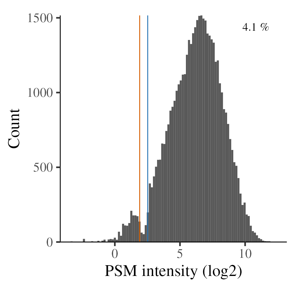
TMT intensities, with notch region denoted by vertical lines
Sub-notch values are systematic under-estimates (currently
unpublished findings). The impact of sub-notch values on summarised
protein-level abundances will depend on the number of sub-notch values
and, more importantly, the proportion of PSMs below the notch for a
given protein. We can obtain the per-protein notch metrics using
get_notch_per_protein and plot the number and fraction with
plot_below_notch_per_prot and
plot_fraction_below_notch_per_prot respectively.
In the case, we see that most proteins have zero PSM intensities below the notch. The vast majority of protein have <10% PSMs at/below the notch, indicating the notch is unlikely to be problematic with this dataset.
notch_per_protein <- get_notch_per_protein(psm)

plot_below_notch_per_prot(notch_per_protein)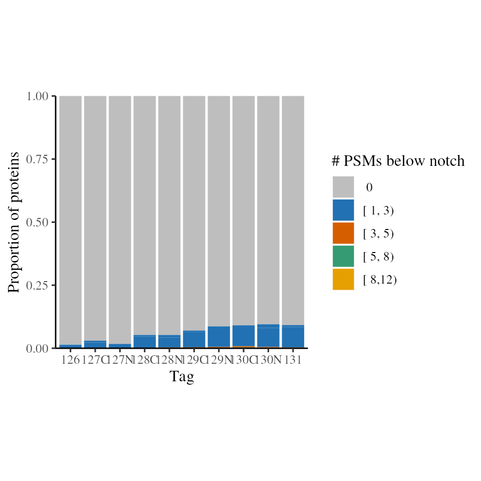
Count of TMT intensities below the notch per protein
plot_fraction_below_notch_per_prot(notch_per_protein)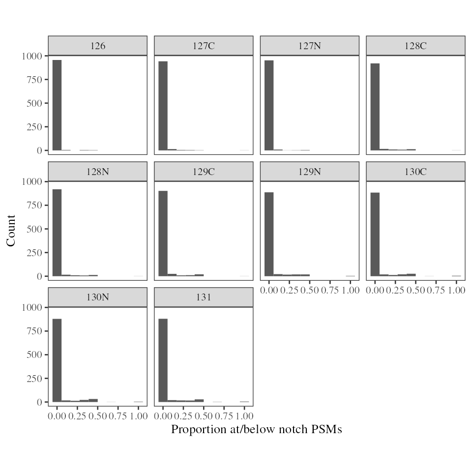
Fraction of TMT intensities below the notch per protein
Removing low quality PSMs
We will still want to remove low Signal:Noise (S:N) PSMs, since the
quantification values will be less accurate and there will be more
missing values and sub-notch values. We can inspect the relationship
between S:N and missing values using the plot_missing_SN
function.
Note that where the signal:noise > 10, there are far fewer missing values.
plot_missing_SN(psm, bins = 27)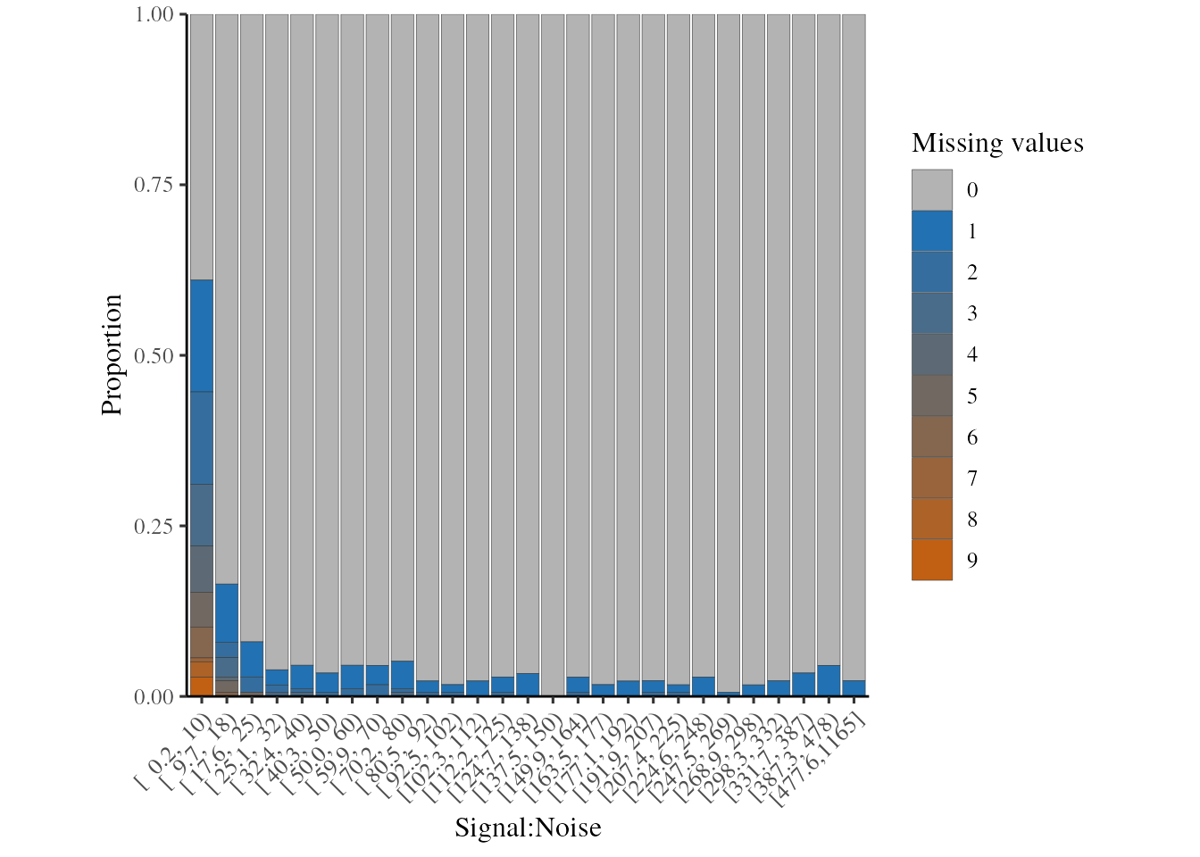
Missing values per PSM, in relation to the signal:noise ratio
We can also look into this relationship at the tag level using
plot_missing_SN_per_sample. In this case, there is no tag
which appears to have a high proportion of missing values when
signal:noise > 10.
plot_missing_SN_per_sample(psm, bins = 27)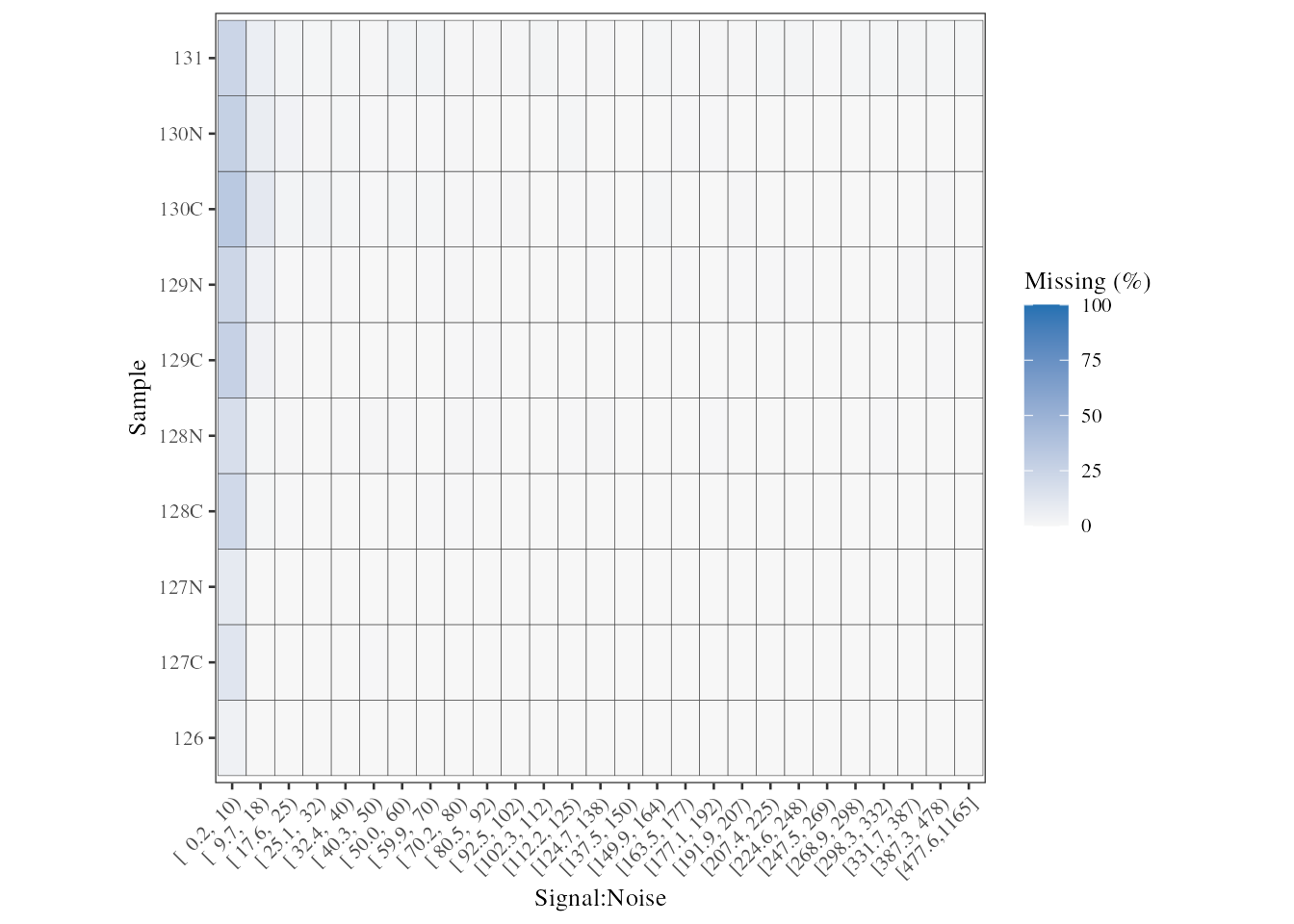
Missing values per tag, in relation to the signal:noise ratio
Based on the above, we will filter the PSMs to only retain those with
S:N > 10 using filter_TMT_PSMs. Using the same function,
we will also remove PSMs with interference/co-isolation >50%.
psm_filt_sn_int <- filter_TMT_PSMs(psm, inter_thresh = 50, sn_thresh = 10)
#> Filtering PSMs...
#> 4747 features found from 2242 master proteins => No quant filtering
#> 4628 features found from 2206 master proteins => Co-isolation filtering
#> 4453 features found from 2174 master proteins => S:N ratio filtering
Summarising to protein-level abundances
Now that we have inspected the PSM-level quantification and filtered the PSMs, we can summarise the PSMs to protein-level abundances.
For PSM to protein summarisation, we will use
MSnbase::combineFeatures(method = 'robust'). This approach
can handle missing values but it only makes sense to use PSMs quantified
across enough proteins and to retain proteins with enough PSMs.
Here, we will use PSMs with at most 5/10 NAs and
proteins with at least 2 finite quantification values in a given sample.
Note that this means a given protein may still have a mixture of finite
and NA values. For example, if a protein has >= 2 PSMs
and the PSMs have missing values such that some samples are still
quantified in all 2 PSMs, then the protein will be quantified in these
samples, but NA where < 2 PSMs have quantification
values. Thus, each protein-level quantification will be derived from at
least 2 PSM intensities, and each PSM will have been quantified in at
least 5 samples.
psm_filt_sn_int_missing <- psm_filt_sn_int %>%
  MSnbase::filterNA(pNA = 0.5) %>% # remove PSMs observed in fewer than half of the samples
  restrict_features_per_protein(min_features = 2)
#> `stat_bin()` using `bins = 30`. Pick better value with `binwidth`.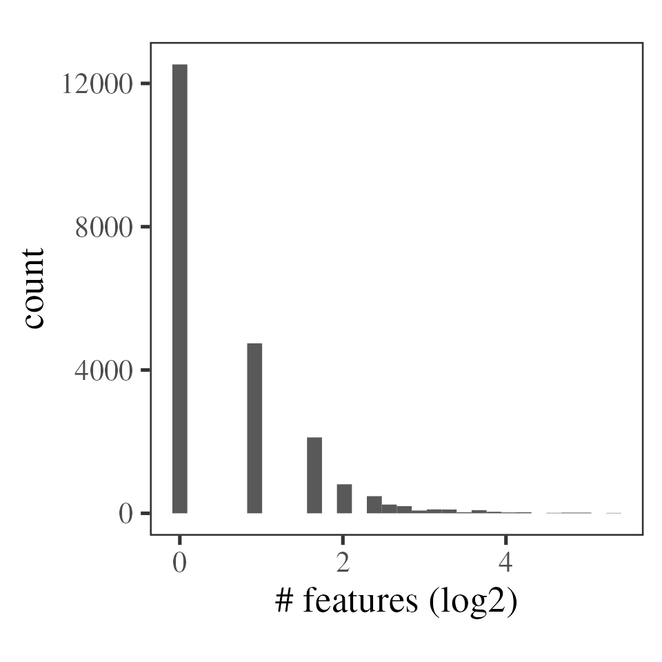
Tally of PSMs per protein
Below, we perform the summarisation. Note that robust summarisation requires log-transformed intensities. If desired, one can exponeniate the protein-level intensities post-summarisation, as shown below.
prot_group <- MSnbase::fData(psm_filt_sn_int_missing)$Master.Protein.Accessions

protein_robust <- psm_filt_sn_int_missing %>%
  log(base = 2) %>%
  MSnbase::combineFeatures(groupBy = prot_group, method = 'robust', maxit = 1000)
#> Your data contains missing values. Please read the relevant section in
#> the combineFeatures manual page for details on the effects of missing
#> values on data aggregation.

Biobase::exprs(protein_robust) <- 2^Biobase::exprs(protein_robust)
Alternatively, one can perform a more typical summarisation to protein-level abundances by simply summing the PSM-level abundances. In this case, we do not want to allow any missing values and will again demand at least 2 PSMs per proteins
psm_filt_sn_int_missing <- psm_filt_sn_int %>%
  MSnbase::filterNA() %>% # remove PSMs with any missing values
  restrict_features_per_protein(min_features = 2, plot=FALSE)

prot_group <- MSnbase::fData(psm_filt_sn_int_missing)$Master.Protein.Accessions

protein_sum <- psm_filt_sn_int_missing %>%
  MSnbase::combineFeatures(groupBy = prot_group, method = 'sum')
Comparing the two summarisation approaches, we can see that the robust summarisation allows us to keep more proteins, since we don’t exlude all PSMs with missing values.